Star rating charts are a type of visualization that can display data like a bar chart, but with stars instead. A common use case for this chart type is for displaying customer satisfaction in product reviews. In this guide, we’re going to show you how to create five-star rating chart in Excel by using conditional formatting.
Data
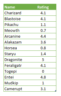
We have a list of items with different ratings. We are going to be using rating values between 0 (bad reviews) and 5 (good reviews) using a five-star rating chart.
Normalizing raw data
If your data set doesn't fit into the same 0-5 range we are using here, you can convert the values into ratings with some additional calculations.

To prepare your data, you need to calculate the maximum and minimum values in the list. You can use the MAX and the MIN functions to do this.

The next step is to find the difference between each interval between ratings. Since there will be a five-star rating chart, we need to divide the difference between minimum and maximum values.

Once you get the interval value, subtract the minimum from the actual data and divide the result by the interval value to find a five-based value.

You can consider rounding the values to fit your rating convention. For example, a value like 0.92 gets a half-star because it is less than 1. On the other hand, you may round the values above 0.5 to 1. Then the value 0.92 will get a full-star.
You can use the ROUND, ROUNDUP and ROUNDDOWN functions to round the values. Alternatively, you can use the CEILING.MATH, FLOOR.MATH and MROUND functions to round by a multiplier.

Creating a five-star rating chart
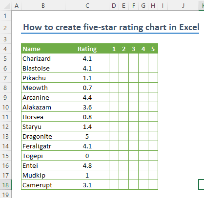
Once the data is ready, you can start adding stars. The trick is to use predefined star shapes with Conditional Formatting. The feature can display a full, half or an empty star in a cell based on the cell value rules. However, each cell can display only a single star. Thus, we need 5 cells for each item.
Our rule will be as follows:
- show a full star if the value is equal or greater than 1
- a half star if the value is equal or greater than 0.5
- finally show an empty star if the value is less than 0.5
So, each cell's value should be equal to the maximum. For example, to display 2.6, the cells should return 1, 1 and 0.6 which can be displayed as 2 and a half stars.
Fortunately, you can generate this numbers using a single formula and a "helper value". First, enter numbers from 1 to 5 in the same column as the ratings. Then adjust and copy the following formula into your worksheet:

You can copy the formula into the entire rating area, but remember to lock the column reference for the data ($C5) and the row reference for the rating (D$4) cells. Otherwise copied cells will have incorrect cell references.
We can now add conditional formatting rules.
- Select the calculated rating values.
- Follow the Home > Styles > Conditional Formatting > Icon Sets path to find the stars.
- Click 3 stars in Ratings section.


You will see the stars added automatically. However, we also need to hide the numbers.

When the ratings are selected, click Manage Rules under the Conditional Formatting menu. Double-click on the rule to open the Edit Formatting Rule dialog.
- Uncheck Show icon only
- Modify the rule based on your rating scale. The default behavior is using percentages.
- Clicking the OK buttons will remove the numbers and adjust the scales if you updated the rule.