Function: MROUND

Excel, with its powerful array of functions, continues to be a cornerstone for data manipulation and analysis. In this guide, we'll delve into the intricacies of the MROUND function, a versatile tool for rounding numbers to the nearest specified multiple. Understanding this function is pivotal for precision in your data calculations. We'll explore its syntax, examples, and equip you with tips and error-handling methods to navigate potential pitfalls seamlessly.

Supported versions

All versions

Syntax

MROUND(number,multiple)

Arguments

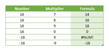
Number	The number to be rounded.
Multiple	The multiple to which you want to round number.

Examples

Firstly a reminder: Named ranges are added to ease of reading formulas.

Example 1

=MROUND(16,9)

formula returns 18. The 9 has 2 multiples near to 16, which are 9 and 18. Because the 18 is the nearest, the formula returns 18.

Example 2

=MROUND(-16,-9)

formula returns -18 according to similar logic with Example 1. On the other hand, if the number is negative, choose a negative number for the multiplier as well.

Download Workbook

Tips

Use the ROUND for standard rounding.
Use the ROUNDUP to always round up.
Use the ROUNDDOWN to always round down.

Issues

#NUM!

If the number and multiplier has opposite signs (+/-), the #NUM! error is returned.

Armed with the insights provided in this guide, you are now well-equipped to wield the MROUND function in Excel effectively. Precision in rounding numbers, along with adept error handling, ensures the reliability of your data analyses. Excel's capability to navigate complex calculations is further amplified by mastering functions like MROUND. As you incorporate these techniques into your spreadsheet endeavors, you pave the way for more accurate and efficient data manipulation.