Excel MATCH function is a lookup/reference formula that returns the relative position of a lookup value from a specified range. The position can be used as the index value in other lookup functions. In this guide, we’re going to show you how to use the Excel MATCH function and also go over some tips and error handling methods.
Supported versions
- All Excel Versions
Excel MATCH Function Syntax
Arguments
| lookup_value | The value whose position index you want to find. |
| lookup_array | The range of cells that contain the lookup value. |
| match_type | Optional. Specifies the match type. The default value is 1. |
Function Match_type
| 1 or omitted | Less than: The MATCH finds the largest value that is less than or equal to the lookup_value. The lookup_array must be sorted in an ascending order. |
| 0 | Exact match: The MATCH finds exact value defined in lookup_value. The order of lookup_array is insignificant. |
| -1 | Greater than: The MATCH finds the smallest value that is greater than or equal to the lookup_value. The lookup_array must be sorted in a descending order. |
Examples of the Excel MATCH Function
Note that we're using named ranges to make the formulas easier to read. This is not required.
#1

#2
The following screenshot shows what value the MATCH function returns when searching for the same value ("Meowth") in lists that contain the same values in a different order.
While the orange cells indicate the correct values, the light green cells have the wrong values or contain errors. Essentially, match_type 1 is best used in lists sorted in ascending, and match_type -1 suits lists sorted in descending order.

#3

Function Tips
- The most common use of the MATCH function is with a lookup function. You can create a dynamic lookup by combining the MATCH function with an INDEX function: INDEX & MATCH: A Better Way to Look Up Data
- An exact search will be typically slower than approximate match types. On the other hand, the approximate search types require sorted lists. For detailed information about lookup function's performances see: How to speed up lookup formulas
- The Excel MATCH function is not case-sensitive.
- Use wildcard characters if match_type is 0 and lookup_value is a text string. Wildcard characters:
| Character | Description | Sample | Meaning |
| ? | Takes the place of a single character | “Admin?” | 6-character word starts by “Admin” |
| * | Can take the place of any number of characters. | “Admin*” | Any number of character word starts with “Admin” |
| ~ | Use tilde in front of a question mark or an asterisk to actually find them | “Admin~*” | Equal to "Admin*" |
Issues
#N/A!
The #N/A error means that no matches were found.