The Excel INDEX function returns a value or the reference of a value at a given position in a range or array. The INDEX function has two different forms to return a value or a reference. Using an array form returns a value, while a reference form returns a reference. In this guide, we’re going to show you how to use the Excel INDEX function and also go over some tips and error handling methods.
Supported versions
- All Excel Versions
Excel INDEX Function Syntax
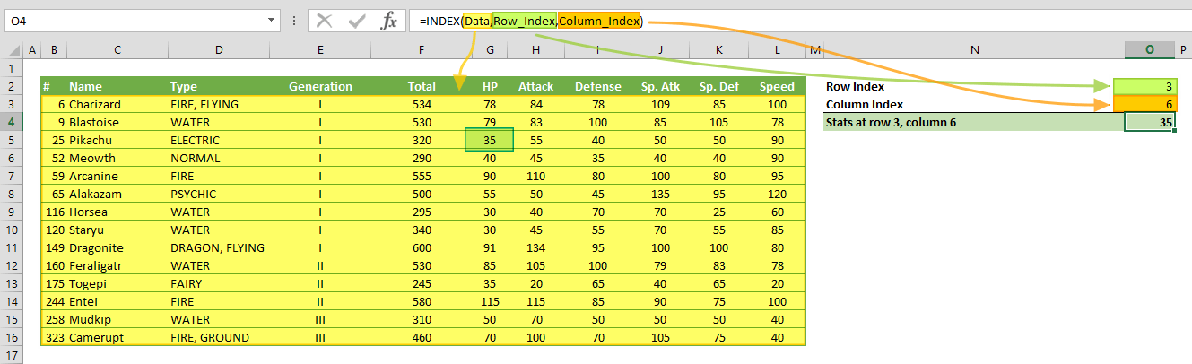
Reference Form: INDEX(reference, row_num, [column_num], [area_num])
Arguments
| array / reference | A range of cells or an array constant. |
| row_num | The position of the row in the reference or array. |
| column_row | Optional. The position of the column in the reference or array. |
| area_num | Optional. Specifies the area that is used in the formula. Areas are numbered by the order they are specified. For example, if reference is (A1:C5,E10:G16) area_num 1 refers the range A1:C5 and area_num 2 refers the range E10:G16. |
Examples
Note that we're using named ranges in our examples to make the formulas easier to read. This is not required.
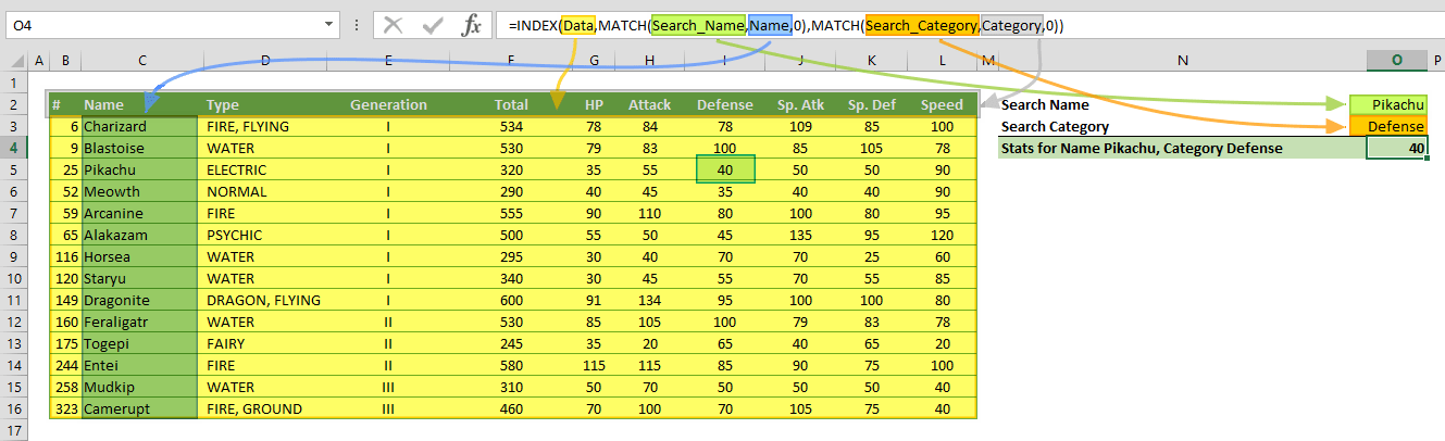
Array Form
Example 1
Example 2
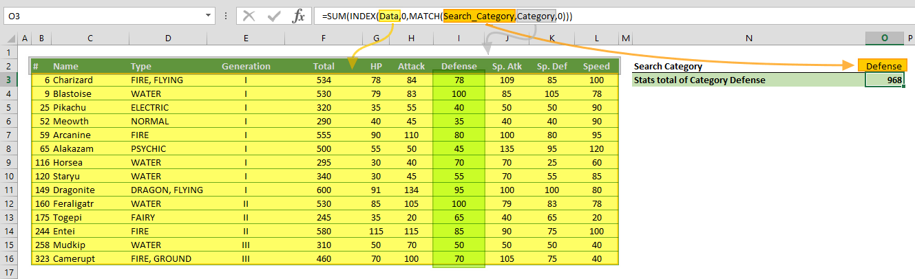
Example 3
In this example, the INDEX returns the values from the Defense column and the SUM function sums these numbers.
Reference Form
Example 1

Example 2

Tips
- The Excel INDEX function can be combined with the MATCH. Combination of the two functions will give you a dynamic lookup approach: INDEX & MATCH: A Better Way to Look Up Data
- If the array argument contains only a single row or column, you can omit the corresponding row_num or column_num argument. For example, formula returns the value from the 3rd column.=INDEX(A1:J1,3)
Issues
#REF!
If values of row_num, column_num or area_num arguments are greater than the specified range, array, or the reference, the formula returns an #REF! error.
#VALUE!
- If area_num is 0, the formula returns #VALUE!
- If values of row_num, column_num or area_num arguments are negative numbers, the formula returns #VALUE! error.