
Spreadsheets move between Excel and Google Sheets constantly. A file gets emailed to someone who lives in the other app, downloaded for a client who does not, or shared with a team split between the two. The natural assumption is that the formula travels intact from one side to the other.
It does not. When a file crosses between the apps, the destination does not simply read the formula; it re-encodes it into its own notation. Most of the time that works and you never notice. The rest of the time, the re-encoding is where things break. And the failure that should worry you most is not the loud one: a converted workbook may open successfully while quietly calculating different business results. The numbers look fine, the file looks fine, and a total is wrong.
This article walks through what actually happens, in both directions, Excel into Google Sheets and then Google Sheets back into Excel. For the behavior differences that exist even without moving a file, see the complete compatibility guide and the worked examples in Same formula, different answer. This piece is about what conversion adds on top of those.
A note on scope: this article focuses on formulas. Charts, PivotTables, VBA, Apps Script, formatting, Power Query, and macros introduce their own compatibility issues that are beyond what we cover here.
How this was tested
The findings below come from direct testing, not from vendor documentation, which says little about these conversions. So that you can judge and reproduce them, here is the setup.
- Excel version: Microsoft 365, version 2606 (Build 20131.20090)
- Google Sheets: web version, tested on July 1, 2026
- Conversion path tested: full conversion to native Google Sheets (Save as Google Sheets, or Drive auto-convert) unless noted; see the callout below on why this matters
- Test workbooks: 5 purpose-built workbooks
- Functions and cases tested: XLOOKUP, UNIQUE, FILTER, SORT, TOCOL, CHOOSECOLS, WRAPROWS, INDEX/MATCH, QUERY, and table columns named with reserved characters
- What was recorded for each: the formula as stored after conversion (from the formula bar), the displayed result or error, and the returned value compared against the source app
Where a claim is an explanation rather than a direct observation, it is marked as inferred. The observable facts are the stored formula text, the error code, and the returned value; the rest is interpretation.
The shapes of failure: a quick map
Almost everything below fits into one of a handful of outcomes. This table is the mental map for the rest of the article.
| Direction | Outcome | Example |
|---|---|---|
| Excel to Google | Clean translation, same result | XLOOKUP |
| Excel to Google | Silent recomputation, different result | UNIQUE (case sensitivity) |
| Excel to Google | Stays in Excel form, then #NAME? |
FILTER, SORT with plain ranges |
| Excel to Google | Stays in Excel form, then #ERROR! |
TOCOL, CHOOSECOLS, WRAPROWS with table references |
| Google to Excel | Array formula re-wrapped in braces | XLOOKUP returns as {=...} |
| Google to Excel | Validation failure, formula stripped to value | a table column named # |
| Google to Excel | Single-value marker added | =B2:B15 becomes =@B2:B15 |
| Google to Excel | No equivalent function | QUERY becomes #NAME? |
The one idea behind all of it
Two differences between the apps cause almost everything in that table.
The first is how each app represents a formula that produces more than one value. Excel uses dynamic arrays that spill into neighboring cells, and it carries an older notation, the legacy array formula wrapped in curly braces and entered with Ctrl+Shift+Enter. Google Sheets uses native dynamic arrays and spilling, with ARRAYFORMULA as its array modifier. Google does use curly braces, but for building array literals inline, not to mark a whole formula as array-entered the way Excel's legacy notation does. The two apps describe the same idea, "this formula yields an array," in incompatible ways.
The second is how each app handles table references. Excel has structured references like Table1[Column], and its syntax reserves certain characters for special meaning. Google has its own table model and does not reserve those characters the same way, so a reference that is legal on one side can be invalid on the other.
Conversion has to translate between these models, and that is where formulas get re-encoded, left in a foreign form, wrapped, or dropped. Everything below is a case of that one idea.
Part 1: Excel into Google Sheets
Read this first: there are two different import paths. When an Excel file reaches Google, it can arrive in one of two ways, and they are not the same. In Office editing mode, the file stays an
.xlsxand Google works on it in place. In a full conversion, through Save as Google Sheets or Drive's auto-convert setting, the file becomes a native Google Sheet. The findings in this section come from full conversion. We have not systematically mapped how each behaves in editing mode, so if your file stays an.xlsx, treat these as a starting point and verify.
Most functions translate and just work
Start with the reassuring case, because it is the common one. The bulk of everyday formulas convert cleanly and return the same answer. XLOOKUP is a good example: an Excel XLOOKUP, even one built on a table, comes through as a working native Google formula with the same result.
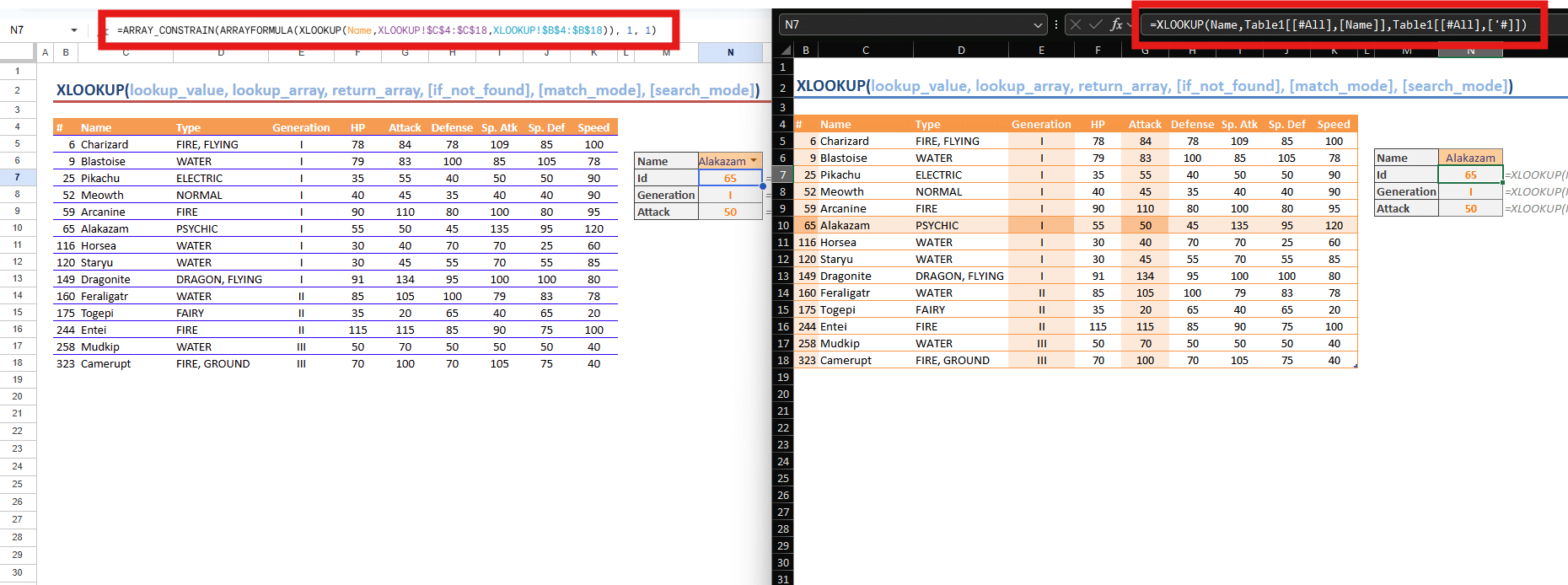
What the converted cell holds matters for the cases that follow. An Excel =XLOOKUP(Name, Table1[[#All],[Name]], Table1[[#All],[#]]) arrives looking like this:
=ARRAY_CONSTRAIN(ARRAYFORMULA(XLOOKUP(Name, XLOOKUP!$C$4:$C$18, XLOOKUP!$B$4:$B$18)), 1, 1)There is no leftover Excel prefix and no table syntax: the function is now native Google, and Table1[[#All],[Name]] has become $C$4:$C$18. The conversion appears to have recognized the function and rewritten both it and its table references. This is the clean path. Hold on to that picture, because the failures are all departures from it.
When it translates but quietly returns a different answer
The most dangerous outcome is the one with no error: the formula converts to a working native form, nothing looks wrong, but the returned value differs because Google computes it under its own rules.
UNIQUE is the clearest case, and the cause is case sensitivity, a documented difference. Google's UNIQUE is case-sensitive; Excel's is not. On a list of Apple, apple, Banana, Excel returns two rows, treating Apple and apple as the same, while Google returns three.

Through a converted file it gets worse, because that recompute collides with the wrapper the conversion added. The converted formula arrives as roughly =ARRAY_CONSTRAIN(ARRAYFORMULA(UNIQUE(...)), 2, 1), where the ARRAY_CONSTRAIN was sized to Excel's two-row result. Google recomputes three rows, the wrapper clips the output back to two, and you are left with Apple and apple while Banana, a genuinely unique value, is dropped. The result matches neither app, and there is no error to flag it.
Natively, case sensitivity just changes a row count. In transit, it can corrupt the result. This clip-and-corrupt behavior is confirmed for UNIQUE; do not assume it for every case-sensitive function without testing.
When it does not translate and breaks loudly
Not every function comes through translated. Based on repeated testing, the set of functions that convert to a native form appears narrower than the set Google's engine actually supports. When a function is not translated, the converted cell still carries its original Excel form, and it errors.
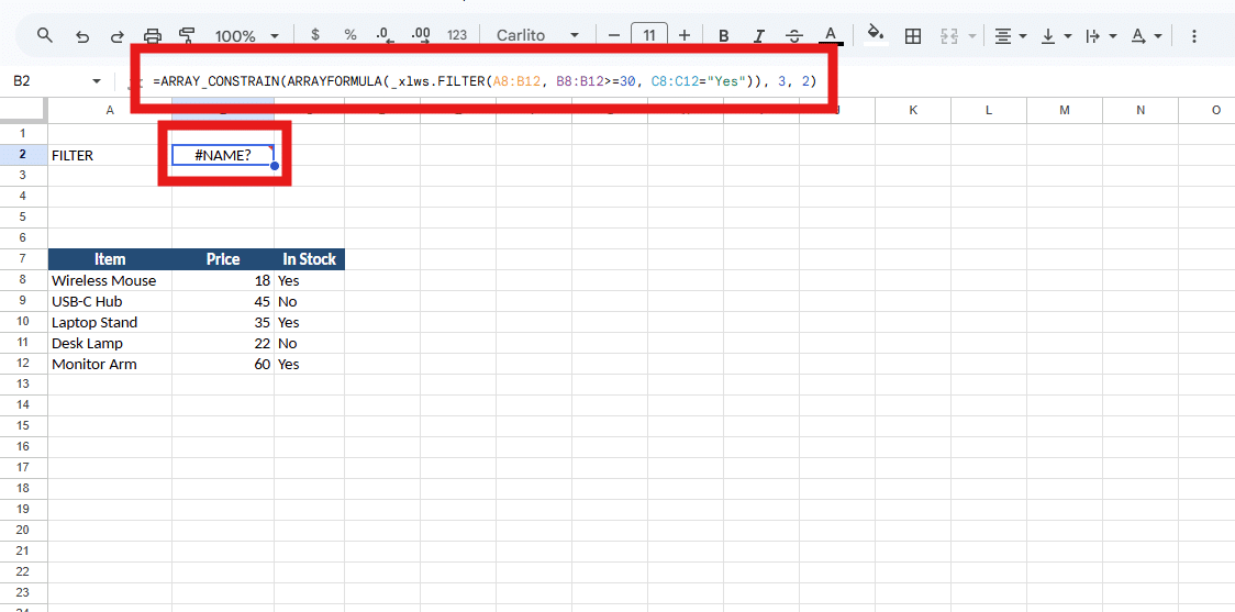
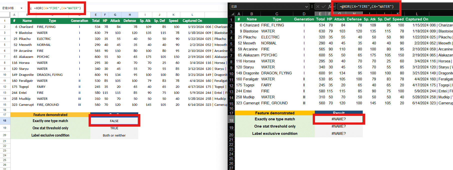
There are two error outcomes, decided by the arguments. If the formula references plain cell ranges, the cell shows #NAME?, because Google's engine does not recognize the stored Excel function name. FILTER and SORT behave this way.
If the arguments include a table reference, the result is worse: #ERROR! instead of #NAME?, because Google's parser cannot read the Excel table syntax at all. TOCOL, CHOOSECOLS, and WRAPROWS behave this way when they reference a table. An Excel =TOCOL(Table2[[HP]:[Speed]]) arrives as:
=ARRAY_CONSTRAIN(ARRAYFORMULA(_xlfn.TOCOL(Table2[[HP]:[Speed]])), 84, 1)and returns #ERROR!.
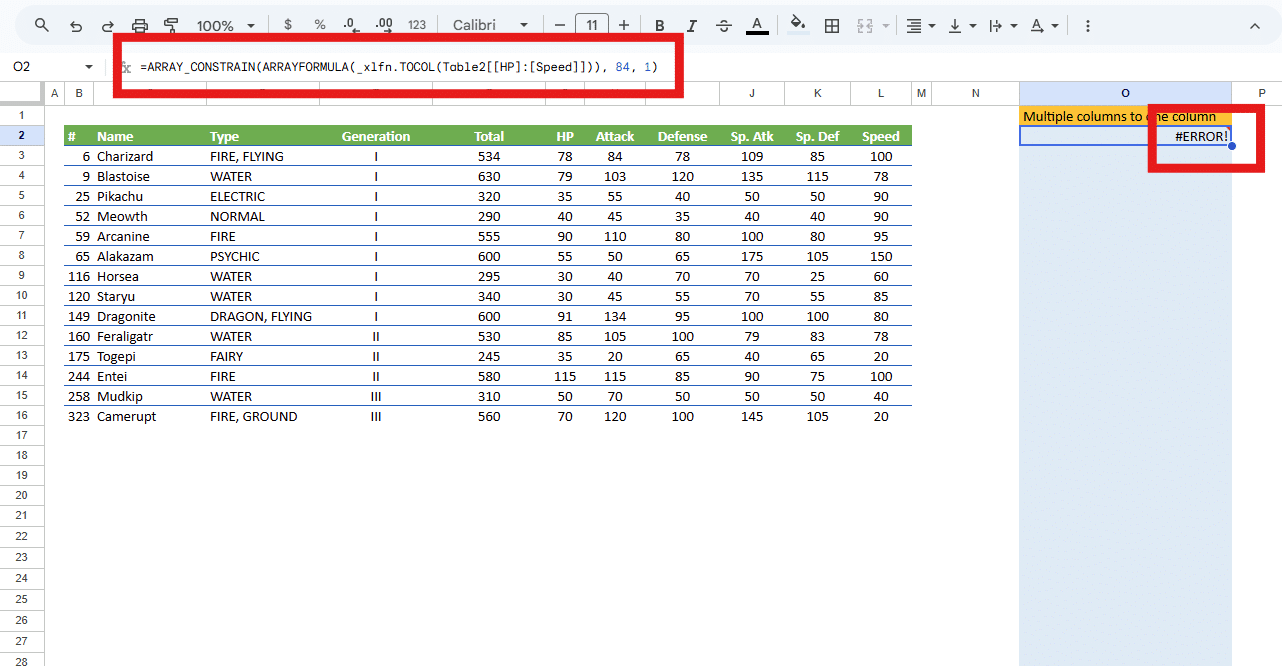
The surprising part is that these functions are not missing from Google. Google natively supports a wide range of array and reshaping functions, including VSTACK, TOROW, WRAPCOLS, CHOOSECOLS, TAKE, and DROP, all of which work when typed directly into a sheet. You can type =TOCOL(G3:L16) into Google Sheets and it works. The gap is in the conversion, not the engine.
Key finding. Google's calculation engine supports TOCOL. Its file conversion does not translate it. A function you could type by hand still breaks when it arrives in a converted file.
The frozen-and-errored outcome is confirmed for TOCOL, CHOOSECOLS, and WRAPROWS. Whether the rest of the family behaves the same way on import is still worth confirming function by function, but their native support is not in question.
What happens to the table references themselves
A natural question is whether the table references are the problem. They are not, and the contrast between the two cases above shows why. When a function is translated, its structured references are rewritten to A1 ranges, as the XLOOKUP example showed: Table1[[#All],[Name]] became $C$4:$C$18, cleanly. When a function is not translated, the whole formula stays in its Excel form and the table reference stays with it, contributing to the #ERROR!. So the structured reference survives fine inside a function that converts, and breaks only when stranded inside one that does not. The deciding factor is the function, not the reference.
The repair trap
There is a follow-on risk that turns a visible error into an invisible one. Faced with a #NAME?, the obvious move is to clean up the formula until the error goes away, stripping the unfamiliar wrappers and retyping it as a plain Google formula. The error clears and the cell returns a value. The problem is that the value is now computed under Google's rules, which, as UNIQUE showed, are not always Excel's. The loud, honest error has been replaced by a silently different answer. If you repair a converted formula, rebuild it deliberately and check the result against the original, rather than just making the error disappear.
What this means in practice. If you send an Excel report to someone who opens it in Google Sheets, the functions that break will usually break loudly, which is recoverable. The real exposure is the function that converts cleanly but recomputes, like UNIQUE, and the formula that someone "fixes" into a silently different answer. Those are the ones that reach a customer wrong.
Takeaway: whether an Excel formula survives the trip into Google Sheets depends on the conversion, not on Google's calculation engine.
Part 2: Google Sheets into Excel
The return trip rhymes with the first half. Where Excel-to-Google stalls on functions the conversion will not translate, Google-to-Excel mostly stumbles on how Google's array model is expressed in the Excel file.
Array formulas come back wrapped in braces
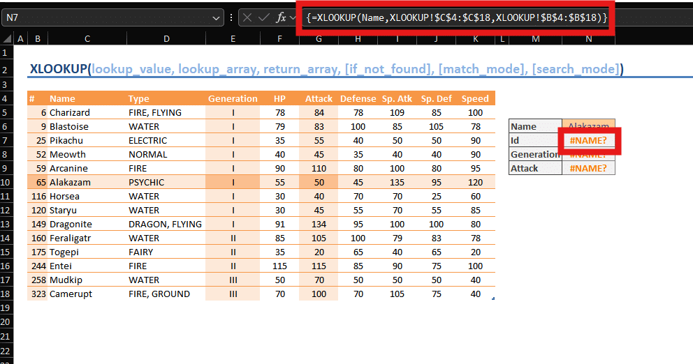
In Excel, a formula wrapped in curly braces is a legacy array formula, the kind entered with Ctrl+Shift+Enter. Google marks its own array formulas with ARRAYFORMULA rather than braces, and where Google uses braces it is for array literals, a different purpose. But in the downloaded Excel file, Google's array-style formulas appear in Excel's legacy braced form, so a formula that was ordinary in Google shows up as {=XLOOKUP(...)}.
Usually the value still computes, but the legacy array form behaves differently from a native one. It sits in a fixed range and does not spill or expand, Excel refuses to let you edit part of it and warns "you can't change part of an array," and in some cases the cell reads blank until you click in and press Enter. A blank cell where a number belongs can be mistaken for missing data. The fix for one cell is to click in, remove the braces, and press Enter, but there is no clean way to prevent the braces on export, which makes it painful across a large sheet. Users report exactly this on both Microsoft's and Google's own support forums.
A harsher failure: the recovery prompt and lost formulas
Sometimes the file triggers a warning on open. Excel reports that it found a problem with some content and asks whether to recover as much as it can. Clicking Yes opens the file but strips the formulas it could not read, leaving only the last values Google had stored alongside them. The observed behavior is consistent with part of the file failing Excel's validation, with the repair keeping what it can parse, the value, and discarding what it cannot, the formula.

This is more alarming than the braces, because the formulas are simply gone afterward, replaced by static values, behind a message that looks like generic corruption.
One confirmed trigger: a reserved character
One reproducible cause of that prompt is a table column whose name uses a character Excel reserves in its structured-reference syntax, and the instructive part is what it reveals.
Consider a Google table with a column named #. The formula =XLOOKUP(Name, Table1[Name], Table1[#]) works in Google. In the downloaded file the reference appears as the bare Table1[#]. But # introduces Excel's special item specifiers, like [#All] and [#Data], so a bare Table1[#] is not valid, the validation fails, the recovery prompt fires, and the formula is stripped to its value.

Now compare a column named @. The formula =INDEX(Table1[@], MATCH("WATER", C2:C15, 0)) comes through as =INDEX(Table1['@], MATCH("WATER", C2:C15, 0)), with the @ escaped by a single quote, exactly the form Excel itself writes for such a name. That formula survives.

Both characters are legal in an Excel column name, and both have a defined escaped form, '@ and '#. In testing, the export produced the escape for @ but not for #.
Key finding. Google's export escapes some reserved characters correctly and not others. A column named
@came through escaped and working; a column named#came through unescaped and broke the formula. The escaping mechanism exists; for#it was not applied.
At the time of testing, the practical consequence is simple: keep # out of column and table names in any sheet that will open in Excel. The @ case survived, but the rest of the reserved set was not checked here, so treat the others as unverified rather than safe.
The @ that appears in front of formulas
A different @ shows up in a different place, at the front of whole formulas, as =@B2:B15. This one is not a defect; it is a faithful translation of a real difference. In Google Sheets, a bare range reference like =B2:B15 in a single cell returns one value; Google does not spill it. In Excel, the same formula spills the whole range. To make Excel reproduce the single value Google would have shown, the export prepends the implicit intersection operator, the @, which tells Excel to return one value instead of spilling. So =@B2:B15 is Google's single-value behavior expressed in Excel's notation, and it belongs in the same family as the braces: the array model re-expressed on the other side.
In many cases the @ form simply returns the single value. In some cases it can produce an error, and removing the @ so the formula spills resolves it. The exact conditions under which it errors rather than returning a value are worth confirming case by case rather than assuming.
Functions that have no Excel equivalent
Google has functions Excel does not, and they cannot survive as formulas. QUERY is the headline example, along with the IMPORT family (IMPORTRANGE, IMPORTHTML, IMPORTXML), ARRAYFORMULA, the REGEX functions, and GOOGLEFINANCE. In Excel these become a #NAME? error or are left frozen on their last value, because there is no function to evaluate.
There is no automatic fix; the work has to be rebuilt with Excel's own tools, for instance Power Query or a PivotTable in place of QUERY.
Things the file format cannot carry at all
Finally, some things are not formulas and do not travel because the format has nowhere to put them. Apps Script automations, certain chart types, and some data-validation and conditional-formatting rules can be lost or altered. This is loss rather than divergence, less likely to produce a wrong number, but it surprises people who expected a faithful copy.
What this means in practice. A Google sheet sent to an Excel user is most likely to arrive with brace-wrapped formulas that look odd but compute, and most likely to fail outright where it used Google-only functions like QUERY. The case to watch for is the recovery prompt, because that one silently converts formulas to values, and a reserved character in a column name is one way to trigger it.
Takeaways: most Google-to-Excel failures come from re-expressing Google's array model in Excel's legacy format. And a column or table name that is legal in Google can break a formula in Excel, so keep reserved characters, especially #, out of names that will travel.
What to do about it
The single most useful habit is to stop trusting the round trip. A converted file that opens without complaint has not necessarily preserved your logic; it may have translated it, left it in a foreign form, wrapped it, or silently recomputed it.
Test the formulas that matter after every move, in both directions, and check the results against the source rather than assuming they carried over. When a converted formula errors, rebuild it deliberately and verify the answer rather than just clearing the error. Keep reserved characters, # in particular, out of table and column names in any sheet that will reach Excel. And where a file lives in both apps over time, treat each crossing as a step that can change behavior, not a neutral copy.
These behaviors are a snapshot. They were observed at the time of writing and may change as either app updates, so re-test anything load-bearing rather than relying on a description that may have aged.
For the behavior differences that exist even before a file moves, see the complete compatibility guide, and for the silent same-formula-different-answer cases with side-by-side screenshots, see Same formula, different answer.
