In this article, we are going to show you how to create a dynamically changing calendar in Excel.
Populate variables
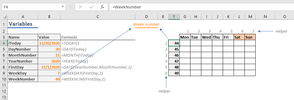
First step is creating the variables to be used in the formulas. These variables need to provide the present day information so that the calendar calendar can update automatically. Here is the list of variables:
- Present date
- The number of the present day of the month
- The number of the present month
- Present year
- The date of the first day of the present month
- The number of the present day of the week
- The number of the present week of the year
We will be using the TODAY, DAY, MONTH, YEAR, DATE, WEEKDAY, and WEEKNUM functions. Briefly, while TODAY function returns the date of the present day, DAY, MONTH, YEAR, WEEKDAY and WEEKNUM functions parse the respective date values. The DATE function returns the date value of the given year, month and day.
In the following screenshot, you can see the names we have given and formulas which were generated on November 20th, 2020.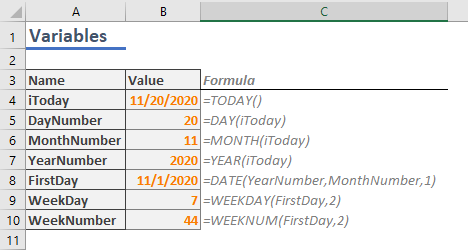
We named each variable to make our job easier when creating formulas. Next step to create a calendar in Excel is creating an outline for the calendar interface.
Outline for the Calendar in Excel
Before creating the actual formulas that generate the days of the month, we first need to place an outline to help creating formulas and also provide visual reference.
The days will be placed on a table of 7 columns and 6 rows. We need to increase these numbers by 2 for titles and helper cells as well. While the column and row titles include week days for columns and week numbers by rows, the helper cells will be consecutive numbers starting from 1.
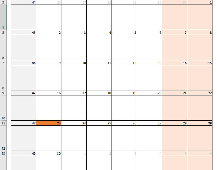
The calendar might look like below.
Use borders or background colors as you'd like. The important point is using a dynamic week number in the title. Reference the WEEKNUM function for the first week, and add 1 for each consecutive week.
| F | |
| 4 | =WeekNumber |
| 5 | =F4+1 |
| 6 | =F5+1 |
| 7 | =F6+1 |
| 8 | =F7+1 |
| 9 | =F8+1 |
Let's continue creating a calendar in Excel by populating the day numbers.
Generating Days
If you are using a similar layout, and don't want to worry about the details of the formula, feel free to copy the formula below. Then paste it into the top-left cell on your calendar’s day area, and populate for the remaining cells. The G2 and E4 cells refer the first cells of the helper columns. Thus, you may need to adjust these references, unless the first cell is G4.

Now, let's take a closer look at the formula. First, the formula uses the DATE function, which returns a date by the given year, month and day. The first 2 arguments are supplied by the variables YearNumber and MonthNumber which have been calculated already.
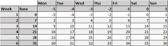
The day part of the formula aims to generate day numbers on a 7-base, since there's 7 days in a week. 7*($E4-1) part of the formula check the week number in the helper column E, and generates a base, starting with 0 and increasing by 7 each time.
| Week | Base |
| 1 | 0 |
| 2 | 7 |
| 3 | 14 |
| 4 | 21 |
| 5 | 28 |
| 6 | 35 |
We can increase or decrease this number as much as the difference between the week day of the first day of the month by the day’s week number. In other words, we are getting the first day of the present month as an anchor point. For example, it is the 7th day of the week (in Monday to Sunday base) for November 1, 2020.
If our calendar’s week assumes that Monday is the first day of the week, Monday should be 6 day before (=1-7) the first day of the month. Thus, we get numbers like below.
| Mon | Tue | Wed | Thu | Fri | Sat | Sun |
| -6 | -5 | -4 | -3 | -2 | -1 | 0 |
Add these values to 1 to shift the numbers. So, Sunday can become the first day like in the following example.
| Mon | Tue | Wed | Thu | Fri | Sat | Sun |
| -5 | -4 | -3 | -2 | -1 | 0 | 1 |
As a result, we have 2 arrays for 2 dimensions. To create a table, we need to add both arrays together.
These numbers represent the day of the present month. There are numbers less than 1 or greater than 31, which obviously can’t be days of the month.
The DATE function handles these types of numbers by generating a date in the previous month or the next. For example, -2 becomes two days before the given month’s first day.
Finally, if you use these numbers in the DATE function, you can get the actual dates of the current month.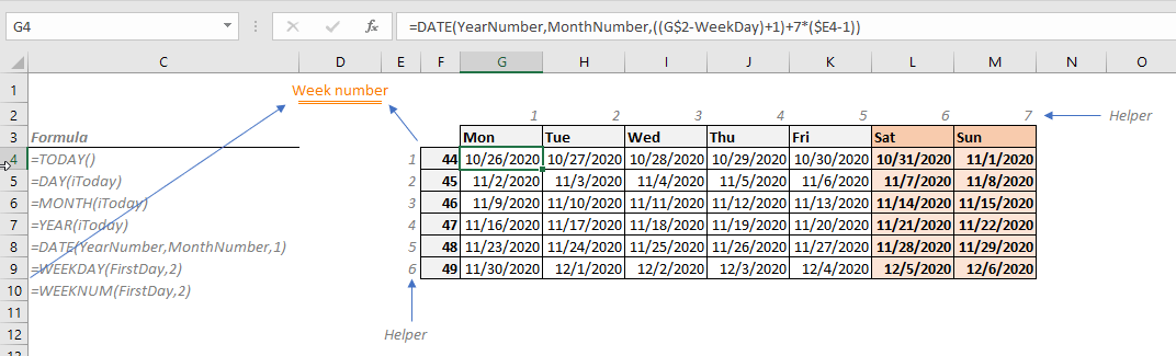
Formatting
Day numbers
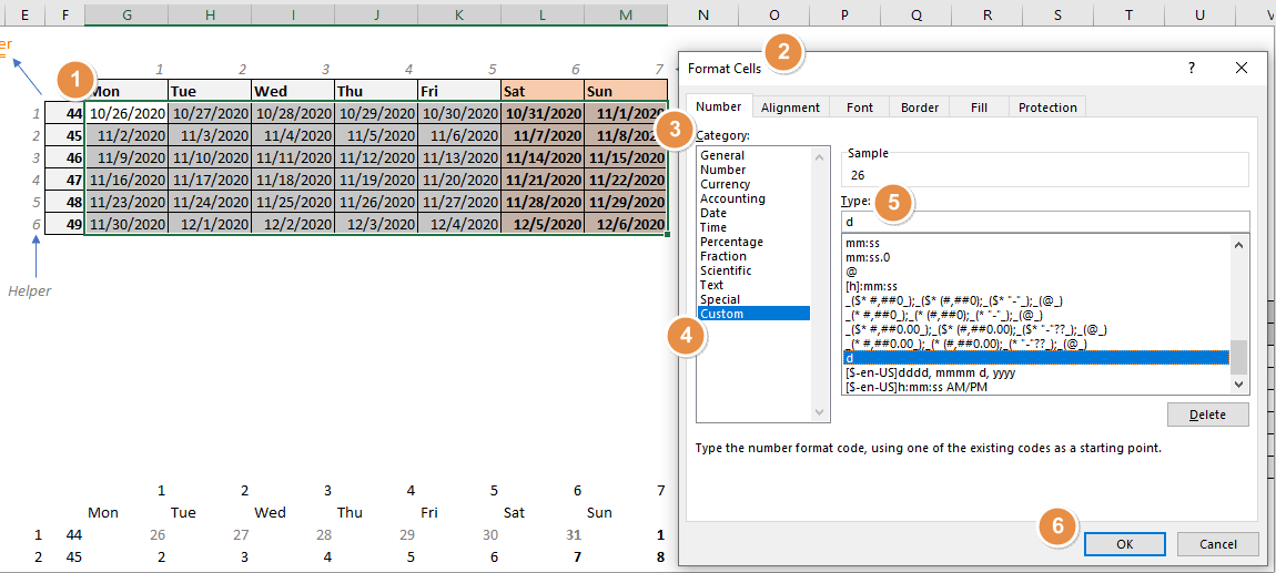
Now, let’s populate the days. You can alter the formatting of the values without changing the actual value. This feature is called Number Formatting. Follow the steps to adjust the number formatting to show only the days.
- Select any the dates in the day area
- Press Ctrl + 1 to open the Format Cells dialog
- Activate the Number tab if it is not open already
- Select Custom in Category list
- Type in the letter d into the Type box
- Click OK to save

Now, the calendar layout is done.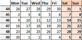
If you want to remove the padding for single digit dates, you can use dd instead of single d. To learn more about number formatting: Number Formatting in Excel - All You Need to Know
Highlighting the present day
Finally, we will be using Conditional Formatting to to set different colors for days that are not in the present month, and highlight the present day.
To add these conditional formatting options;
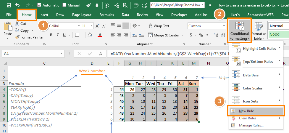
- Select the day range
- Click the Conditional Formatting icon under the Home tab of the Ribbon
- Select New Rule

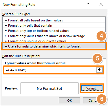
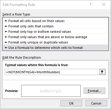
- Select Use a formula to determine which cells to format
- Enter a formula to define the rule for highlighting the current day
=G4=TODAY()
G4: Top-left cell of the range includes days. Use a relative reference (do not use $). - Click the Format button in the Preview window of the Format Cells dialog

- In the dialog, select formatting options you want to see in the present day’s cell
We used an orange background in this example. - Click OK to apply

- The Preview box will display your preferences
- Click OK to apply conditional formatting


This is how it looks: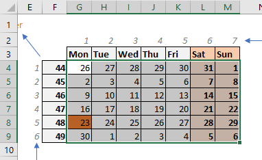
The formula returns a Boolean value. If the cell value (G4) is equal to result of TODAY function, which returns the present day in a date format, the formula returns TRUE. Otherwise, FALSE. If the result is TRUE, Excel applies the formatting into the cell.
There are 2 important points here:
- You need to use a relative reference, e.g. G4, unless you do not want Excel to populate the reference along the range. Consider how formulas change when you copy them elsewhere. Excel applies the same for conditional formatting formulas as well. For more information, see: How to create an Excel absolute reference and relative reference
- The day cells must return the actual date values. This is why we are using number formatting to show the day portions.
Eliminating the days not in the present month
Here is the formula to give a different formatting for days that are not in the present month. They will be grayed out in our example:
Final step is hiding the helper columns.
This is the finale: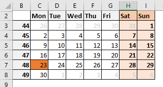
This is how you can create a dynamically changing calendar in Excel.