Duplicate values in a dataset can cause headaches if you do not know how to deal with them. In this guide, we're going to show you how to find duplicates in Excel and also go over how you can remove or consolidate them using a few examples.
How to find duplicates in Excel
If you only want to locate the duplicate values, highlighting them is probably the easiest way to do so. With only two steps, you can change the color of the cells that have duplicate values. Let's see how you can do this using an example.
First select the range of your data (You can select a range or a list).

In the Ribbon, follow the path Home > Conditional Formatting > Highlight Cell Rules > Duplicate Values

Clicking the Duplicate Values item pops a dialog with more options. You can select between highlighting duplicate values or unique values in a specific style.

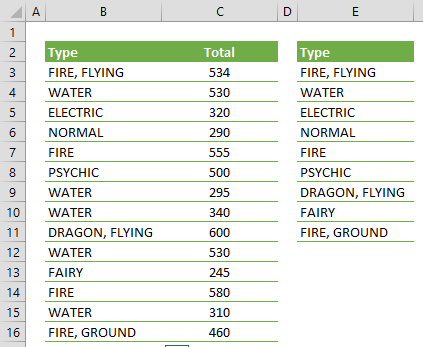
Clicking the OK button applies the specified formatting to the selected range. In our list, "WATER" and "FIRE" values are listed more than once.

The good thing about this method is that Conditional Formatting works with every calculation. Thus, you don't need to update this feature every time you get new duplicates. Let's continue with how you can remove those duplicate values.
How to remove duplicate values
After you find duplicates in Excel, you can select rows one by one and delete them. However, the manual approach obviously might take too long if there is a lot of duplicates. Fortunately, you can use the Advanced Filter feature to remove them at once. Also note that this method is suitable if duplicate values reside in the same column.
Once again, start by selecting the column that contains the duplicate values. But this time, activate the Data tab in the Ribbon, and click on the Advanced icon from the Sort & Filter section. This action pops the Advanced Filter dialog.

In the Advanced Filter dialog, make sure that the Unique records only option is checked. Also, you can enable populating the filtered results on another range. Otherwise, Excel filters the results by hiding duplicate rows. To remove them completely, select Copy to another location option and select a cell for the Copy to range field.

Clicking the OK button populates a list of unique values in the target location.
Now you can use formulas with unique values to consolidate data from your data set. If you want to use formulas to do this instead, please see Pivot Table Alternative Using Formulas. Alternatively, you can also use Excel's Consolidate feature. Next, we're going to take a look at how you can use the Consolidate feature.
How to consolidate duplicate values
Consolidation can be done in many ways in Excel. Formulas like SUMIFS or COUNTIFS are frequently used to do this. You can also use an advanced tool like Pivot Table or Power Pivot for the same effect. As another alternative, Excel has a relatively less-known tool which is designed specifically for this job. Let's see how you can use the Consolidate Tool.
This time, select a suitable cell where the consolidated data is to be populated.

Once again, activate the Data tab in the Ribbon. Click on the Consolidate icon under the Data Tools section to open the Consolidate dialog.

In the Consolidate dialog, you can
- choose a function type which determines the consolidation method,
- add references to be consolidated
- determine label location
- and create links to the source data if it is located in an external target.
Start by determining a function type. Next step is adding the data into references. Activate the Reference field, and select the range that contains the data.

Click the Add button to add the reference into the All references box. Check either Top row or Left column options depending on how your data is structured. We checked both options in this example, because both the top row of our data, 2nd row, and left column, column B, contain labels.

Click OK when you are done. You will see that the consolidated values are populated starting from the selected cell.

That's all! Note that your settings will be saved into the file, so you can repeat this when the data is updated.