Microsoft's data analysis tools PowerPivot, Power BI Desktop, and SQL Server Analysis Services (SSAS) Tabular models empower Excel users by allowing them better manage and transform their data. Data Analysis Expressions (DAX) is essentially a formula and query language for this tool suite.

DAX queries can contain functions, operators, and constants that can be used to define custom calculations for Calculated Columns and for Measures (also known as calculated fields).

Calculated Columns and Measures are two useful features that can help when working with relational data, and performing dynamic aggregation to restructure data that already exist in your model. We will come back to this later. Now let’s take a look at how DAX formulas work and how you can use them to organize your data. You can download our sample workbooks below.

DAX Formulas

Overall, DAX functions are pretty similar to Excel formulas. They use the similar syntax structure - a DAX formula starts with an equal sign, is then followed by a function name or expression, and any additional values or arguments. DAX and Excel share some formulas as well. For example, the SUM and AVERAGE functions, or date-time functions like DAY, MONTH, and YEAR are available in both.

Now, let’s take a look at the differences of the two:

• DAX functions do not use A1 or R1C1 references like in Excel formulas. Therefore, you can't use a range with custom dimensions. The reference must always be an entire column or a table.
• DAX lookup functions require an established relationship between the respective tables.
• While Excel evaluates date and time values as numbers, DAX evaluates them as datetime Functions also show some difference in values returned.
• DAX functions can return a complete column or table, as well as a single value.

Below is the breakdown of a DAX formula:

This formula uses the IF function, which has the same syntax as its Excel counterpart. The data fields End of Year Assets and Average Assets targeted here are coming from the table ‘Breakdown’. You can find this table in the SampleData.xlsx file. The formula compares the two and gives a result ‘Good’ or ‘Bad’. More specifically:

1. The formula starts with an equal sign.
2. The string after the equal sign specifies the calculation method.
3. Arguments are entered inside parentheses.
4. The first argument of the IF function is a logical test that determines which argument is to be returned. The first argument includes a greater than or equal condition between the two columns. Table names comes first as sheet names in Excel and column names follow the table names by located between square brackets. This notation is similar to Excel's cell references as well.
5. Each argument is separated by commas.

Where to Use Them

You can create and use DAX formulas in Power Pivot either in calculated columns or measures. Power Pivot is an Excel add-in created by Microsoft to help users analyze data and create data models. For more details see: Here is How You Can Crunch Data of Any Size with Excel’s PowerPivot

Calculated Columns

A calculated column is essentially adding a new data column into your Power Pivot table. Instead of copying or importing static values into a column, you can create a column dynamically using DAX formulas. Calculated columns can be used in other formulas, just like any other column. Furthermore, they can also be used with Filters, Rows, and Columns features, and the Values area of Pivot Tables using an aggregation method.

The formulas are applied to all columns and are calculated row by row. The results are updated when the data is refreshed.

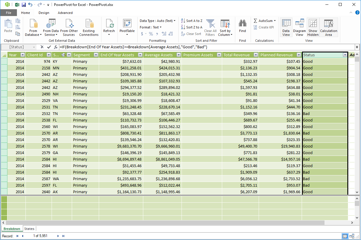
Let’s take an example. Here, the Status column on the right is a calculated column that contains the IF formula we used before in the syntax breakdown.

=IF(Breakdown[End Of Year Assets]>=Breakdown[Average Assets],"Good","Bad")

The result is calculated for all rows and corresponding results for each row are returned in the resulting column. To differentiate from static columns, calculated columns are shown in bold text.

Measures

Measures or calculated fields are the alternative way to use formulas in a data model. Instead of calculating the results row by row, measures perform aggregate calculations. Measures are suitable to use in Values area of a Pivot Table as is without needing to select an aggregation method. However, they can't be used in other areas.

When a column is used in the Values area of a Power Pivot table, Excel implicitly creates a measure that uses the column in an aggregate function. For example, if you move the Planned Revenue field and select SUM for aggregation method, Excel will create a =SUM([Planned Revenue]) measure.

Let's take a closer look at when and why measures are used. In the formula example, we compared End Of Year Assets and Average Assets fields and returned a value. Let's assume that we need the ratio of the two values this time. The easiest way to this is to divide the two. However, if there’s duplicate data in a category, you might want to work with aggregate values instead.

Measures are stored in cells at the bottom section. Coordinates of these cells don't hold any significance, so feel free to use any one of them.

Measure formulas contain one more element. You need to type in the name of the measure and place a colon before the actual formula. Below is an example.

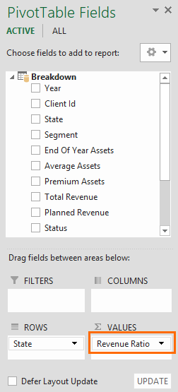
Revenue Ratio:=SUM([Total Revenue])/SUM([Planned Revenue])

The "Revenue Ratio" is the name of the measure we created and the following string is the formula we used before. Here, we also used the SUM function to aggregate values from the entire column before dividing them. Here is how it looks in the Power Pivot window.