Dynamic arrays in Excel mark a significant leap in the functionality of one of the world’s most widely used spreadsheet tools. Introduced in Excel 365 and Excel 2019, dynamic arrays bring a new level of efficiency and power to data manipulation and analysis. This feature allows users to create formulas that not only return multiple values, but also automatically resize and adapt as the data changes. The introduction of dynamic arrays is particularly notable as it simplifies the processes that previously required complex, multi-cell array formulas or VBA programming, making advanced Excel features more accessible to a broader user base.
Unlike static arrays in Excel, dynamic arrays can automatically spill results into adjacent cells, eliminating the need for manual cell range specification. This feature not only simplifies formula creation but also enhances the adaptability of dynamic arrays in diverse computing environments. The ability to spill results is particularly useful in scenarios where the size of the output is not predetermined, allowing for real-time data expansion and contraction.
The concept of a dynamic array is distinct from that of a traditional array in several ways. While a traditional array has a fixed size, determined at the time of its creation, a dynamic array can grow or shrink during runtime, providing a level of flexibility that static arrays cannot match. This dynamic resizing is critical in applications where the volume of data is variable or unknown in advance.
In the context of programming and data analysis, understanding the distinction between dynamic and static arrays is crucial. Dynamic arrays offer advantages in terms of memory management, scalability, and ease of use, making them an ideal choice for a wide range of applications, from simple data storage to complex algorithmic implementations.
Dynamic arrays can populate a range of cells from the values of an array. With dynamic arrays, any formula that returns an array of values will spill the results into the adjacent empty cells automatically. You can create tools like interactive pricing applications with ease.

This feature is meant to replace the existing array formulas (also known as Ctrl+Shift+Enter) formulas.
Expanding on the transformative nature of dynamic arrays in data processing and formula application, it's crucial to understand how they are poised to redefine the traditional approach to array formulas, commonly known as Ctrl+Shift+Enter (CSE) formulas. Dynamic arrays are not just an incremental improvement; they represent a paradigm shift in how array formulas are conceptualized and implemented in various computing environments.
The advent of dynamic arrays marks a significant departure from the constraints and complexities traditionally associated with CSE formulas. In the standard array formula setup, users often encounter limitations related to fixed-size arrays and the cumbersome process of applying formulas across multiple cells. These restrictions can lead to inefficiencies and errors, particularly in complex data analysis tasks.
Dynamic arrays, however, eliminate these hurdles by introducing a more streamlined and intuitive approach. One of the most striking advantages of dynamic arrays is their ability to overcome the restrictions imposed by traditional methods. They simplify the process of working with array formulas by allowing a formula to be applied to a single cell, which then dynamically spills the results across a range of adjacent cells. This spilling behavior is automatic and adjusts in real-time as the underlying data changes, ensuring that the output remains accurate and up-to-date.
Moreover, dynamic arrays enhance the user experience by making array formulas easier to write, understand, and maintain. The elimination of the need for CSE entry simplifies the learning curve for new users and reduces the likelihood of errors for seasoned professionals. This user-friendly nature of dynamic arrays is a game-changer in data processing and analysis, opening up new possibilities for efficiency and creativity.
New Dynamic Array Functions
The introduction of dynamic arrays in Excel is complemented by a suite of powerful new functions, each designed to harness and extend the capabilities of this feature, transforming how users interact with and analyze data. These functions—FILTER, SORT, UNIQUE, SEQUENCE, and RANDARRAY—are not just additions to the Excel function library; they represent a fundamental shift in the approach to data manipulation and analysis within spreadsheets.
FILTER Function
FILTER function allows users to filter data based on specific criteria, dynamically updating the output as the source data changes. For example, you can easily display all rows in a dataset where a certain condition is met, like sales exceeding a certain threshold. This makes it far simpler to create responsive, live dashboards and reports that adjust as new data is added or existing data is modified.
- Syntax: =FILTER(array, include, [if_empty])
- Example: =FILTER(A2:B10, B2:B10>20) filters the range A2:B10 to show only the rows where the corresponding value in column B is greater than 20.
UNIQUE Function
UNIQUE function extracts unique values from a range, eliminating duplicates. This is extremely helpful in data cleaning and preparation, allowing for quick identification and extraction of distinct values from a list. Whether you’re dealing with a list of products, customers, or transactions, UNIQUE ensures that you can easily handle and analyze data without redundancies.
- Syntax: =UNIQUE(array, [by_col], [exactly_once])
- Example: =UNIQUE(A2:A10) lists unique values from the range A2:A10.
SORT Function
SORT function allows to sort data in ascending or descending order without manual intervention. This function is particularly useful for organizing large datasets, ensuring data is always presented in a logical, easy-to-understand format. It becomes incredibly powerful when combined with other dynamic array functions, offering sorted views of filtered or unique data sets.
- Syntax: =SORT(array, [sort_index], [sort_order], [by_col])
- Example: =SORT(A2:B10, 2, -1) sorts the range A2:B10 based on the values in column B in descending order.
SORTBY Function
SORTBY allows you to sort one array based on the values in another array. This feature is particularly useful when you have two related columns of data and you want to sort one column (array) based on the values in the other column. For instance, if you have a list of products and their corresponding sales figures, you can use SORTBY to sort the list of products based on the sales figures, without mixing up the relationship between products and their sales.
- Syntax: =SORTBY(array, by_array, [sort_order], [by_array2, sort_order2],...)
- Example: =SORTBY(A2:B10, B2:B10) sorts the range A2:B10 based on the values in B2:B10.
SEQUENCE Function
SEQUENCE function generates a list of sequential numbers, which is highly useful for creating custom indexes, timestamps, or for any situation where you need a quick series of numbers. SEQUENCE can dynamically adjust the length of the sequence based on other variables or conditions in your workbook, providing a flexible tool for various numerical tasks.
- Syntax: =SEQUENCE(rows, [columns], [start], [step])
- Example: =SEQUENCE(5) creates a single column array with 5 rows containing the numbers 1 to 5.
SINGLE Function
SINGLE function is designed to return a single value from a cell or a range that might contain a dynamic array. This function is particularly useful when you're dealing with formulas that return dynamic arrays, but you need to isolate and work with just one value from that array.
- Syntax: =SINGLE(array)
- Example: =SINGLE(A1:B2) would return the value in the top-left cell of the specified range if used in a formula that expects a single value.
RANDARRAY Function
RANDARRAY function generates an array of random numbers, useful for simulations, random sampling, or any scenario where you need a set of random values. Like SEQUENCE, its size can dynamically adjust, and when used in conjunction with other dynamic array functions, it can provide random sorting, filtering, or selection within a dataset.
- Syntax: =RANDARRAY([rows], [columns], [min], [max], [integer])
- Example: =RANDARRAY(3,3) generates a 3x3 array of random numbers between 0 and 1.
Operators in Dynamic Array Functions
Spill Operator (#)
The Spill operator (#) in Excel is a critical component of dynamic array functionality, significantly enhancing the way formulas handle multiple values. This operator is used to reference the entire range of cells that a dynamic array formula automatically fills, known as the spill range. When a dynamic array formula is entered into a cell, it may produce multiple values that overflow, or "spill," into adjacent cells. The cell where the formula is initially entered is termed the "spill anchor." To reference the entire array of cells populated by this formula, the spill operator is appended to the address of the spill anchor. For example, if you enter a dynamic array formula in cell A1 and it spills over into multiple cells, you can reference the entire range of these cells using A1#. This feature allows for dynamic adjustment of the spill range, automatically resizing based on the data output of the formula, which is especially useful for handling data sets that change in size.
The spill operator greatly simplifies the creation and management of array formulas, marking a significant advancement in Excel's capabilities. It not only helps avoid common errors, like the #SPILL! error which occurs when the spill range is obstructed, but also seamlessly integrates with other Excel functionalities. For instance, spill ranges can be used in charts, PivotTables, data validation, and conditional formatting, enhancing the overall utility of dynamic arrays in data analysis and reporting. Prior to the introduction of dynamic arrays and the spill operator, achieving similar results required complex and often cumbersome array formulas. The spill operator has streamlined this process, making powerful data manipulation tools more accessible and intuitive for users, regardless of their expertise level in Excel.
Single Operator (@)
The Single operator (@), known as the implicit intersection operator, plays a unique role in Excel, particularly in the context of dynamic arrays and legacy array formulas. Originally, the @ operator was used in Excel to handle situations where a formula might return multiple values, but only a single value was expected or required. This was especially relevant in older versions of Excel before the introduction of dynamic arrays. In those versions, array formulas were entered using Ctrl+Shift+Enter and could potentially return multiple values. If such a formula was used in a context where only one value was allowed, the @ operator would ensure that only the first value of the array was considered, effectively performing an "implicit intersection" of the array with the row or column it was in.
With the advent of dynamic arrays in newer versions of Excel, the role of the @ operator evolved. Now, it serves a slightly different purpose: to handle compatibility with older formulas and to manage specific instances where a dynamic array formula is used in a context that requires a single value. For instance, if you have a dynamic array formula that spills over multiple cells and you reference that formula in a cell that can only handle a single value (like a cell used in a data validation rule or a conditional formatting formula), the @ operator can be used to ensure that only one value from that array is returned. This is particularly important for maintaining backward compatibility with older versions of Excel and for ensuring that legacy spreadsheets continue to function correctly without modification. The @ operator, in this way, serves as a bridge between the traditional array formula behavior and the new dynamic array functionality, providing flexibility and control in how formulas are interpreted and executed in various contexts.
Error Handling in Dynamic Array Functions
With the advent of dynamic arrays, Excel also introduced several new error messages. These messages are designed to help users quickly identify and resolve issues specific to the use of dynamic arrays. Some of the new error messages include:
#SPILL! Error: This occurs when a dynamic array formula is blocked from spilling its results by existing data in adjacent cells. It alerts the user to clear the obstructing data to allow the formula to function correctly.
#CALC! Error: This error message indicates a problem with the calculation, often due to complex or circular references within dynamic array formulas. For example, =UNIQUE({2,2,3,3,3,4,4,4,4}, ,TRUE) formula returns #CALC! error because there isn’t any value in the array that occurs once.