What’s a VLOOKUP in Excel?

VLOOKUP is a well-known Excel formula that can save you hours over performing the same tasks manually.  This handy function – as the name VLOOKUP suggests – will allow you to perform vertical lookups to search for specific data. The V stands for vertical, signifying the means by which Excel will search for your data. Vertical lookups are like navigating through a phone book: when you search for a number, you first look for the target name in the leftmost column. Upon finding the name, you will move your finger to the right in order to match the column that contains the phone number, which is the target information. The VLOOKUP in Excel works the same way.

Before we begin, it is recommended that you download the sample workbook, since we will be using it to demonstrate how this functionality works.

Download Workbook

Lead by Example

Excel's VLOOKUP function is a powerful tool that simplifies the process of retrieving data from large datasets, making it an indispensable feature for anyone working with spreadsheets. In this comprehensive guide, we will walk you through the intricacies of using the VLOOKUP function in Excel. From understanding the syntax and parameters to exploring real-world examples, you'll gain a solid grasp of how to leverage this function for efficient data lookup and analysis.

Understanding the VLOOKUP Syntax:

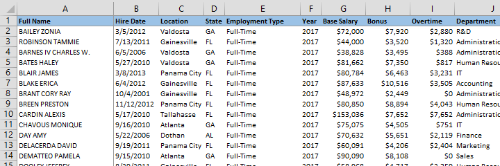
To illustrate the functionality of the VLOOKUP function, let's consider a practical example: retrieving the salary of an employee from a sample list. In essence, we need to search for the employee's name in the Full Name column, identify the corresponding row, and extract the salary from the Base Salary column.

When constructing a VLOOKUP formula, Excel provides a helpful tool called IntelliSense. As you begin typing "=VLOOKUP" into a cell and add the opening parenthesis, IntelliSense guides you by displaying placeholder parameter text bubbles, making the formula-building process intuitive.

Parameters of the VLOOKUP Function:

1. lookup_value: The first parameter signifies what you are searching for. In our example, this is the employee's name, analogous to finding a person in a phonebook.
2. table_array: The second parameter defines where Excel should search for the information. This is akin to specifying the range or table where the data resides, such as columns A through J and all rows on the Employee Data sheet.
3. col_index_num: This parameter represents the information you are seeking—such as the Base Salary in our case. It must be specified as a column index, indicating the position of the desired information in the chosen range.
4. [range_lookup]: The final parameter, an optional Boolean, determines whether to perform an approximate or precise search. Using 0/FALSE or 1/TRUE, you can specify the search type. In most cases, FALSE is preferred for precise searches, especially when dealing with non-numerical values.

Real-World Application:

Let's delve deeper into a practical example to solidify your understanding. Imagine you have an Excel sheet with employee data, and you want to use VLOOKUP to find the salary of an employee named John Doe.

Now, let’s get down to finding the salary of an employee. We are going to be looking for employee “Bates Haley” in this example. The sample workbook contains a sheet dedicated to our search and we can type our formula into the Base Salary box.

Step by step, let’s fill out the formula:

1. First, we are going to add the value (or cell reference of the value) that we want to look up (lookup_value). Our first argument is in cell C1, which is where we are going to type in the Full Name of the employee that we want to find.
2. Next, we need to add the range or the table reference for our data. Remember: VLOOKUP always searches in the first column of your range selection. In this example, we will select the range as A1:J50 (table_array).
3. Excel can now find the name we are looking for. However, we still need to indicate what data we would like returned to us. To do this, we enter the index of the column (col_index_num) which contains the result value in the data range/table we selected. Since we want the formula to give us the Base Salary of this employee, we need to enter 7 (column G). The indexing in Excel begins with value 1 from the left-most column in your range (in this case, Column A). The index increases by 1 for each column to the left (e.g. in this case, B = 2, C = 3, D = 4). IMPORTANT: The column we are searching in (Full Name) needs to be to the LEFT of the column we are searching data in (Base Salary). In other words, VLOOKUP can only start looking for a name on the left, and then return data that is to its right!
4. Lastly, we need to tell Excel whether we are looking for an approximation or a precise value. Adding FALSE (or 0) as [range_lookup] argument will work in most cases as it indicates an exact search. We suggest using FALSE unless the first column of your data contains sorted numerical values (especially if they are formula calculated, rather than static data) and you need to search for numbers.
5. By clicking Enter, we will see that the Base Salary of Bates Haley is $81,662.

Oh no – something went wrong! Common VLOOKUP Mistakes

Your data is ready, you just wrote your formula, you press Enter, and Excel gives you one of its #hashtags instead of a proper result. This list of common errors can help you diagnose the problem when using a VLOOKUP!

#N/A – When using [range_lookup] with approximate (TRUE), the search parameter (lookup_value) might be smaller than the smallest value in the first column of our search area (table_array). Typos or additional spaces in the lookup data are common mistakes that may cause this error.

#REF! – This error typically occurs when the index of the data we are looking for (col_index_num) is greater than the number of columns in our table. Another reason might be missing references in the VLOOKUP formula, such as removing the data table.

#VALUE! – If you try entering a value less than 1 for the search area (table_array), you get this error.

#NAME? – Typically, you get this error if you are missing any quotation marks in the formula. For example, if you’re specifically looking for “Bates Haley”, you should enter

=VLOOKUP(“Bates Haley”,B2:E7,2,FALSE)

That wasn’t so hard!

Searching through vast amount of data in Excel can be extremely tedious if you don’t utilize certain formulas. VLOOKUP allows you to identify and index information extremely easy and, contrary to popular belief, is not hard to implement. Once you understand the logic behind generating the formula’s syntax, we are confident that you will use it at every opportunity. Follow us for more tutorials and don't forget the check the Microsoft's official website!