
The GROUPBY formula in Excel is a dynamic array function introduced in 2023. It allows you to group rows of data based on one or more criteria and perform calculations or aggregations for each group. Essentially, it helps to summarize data by organizing it into meaningful groups, similar to the functionality provided by PivotTables, but with more flexibility and customization.
Why Use GROUPBY Instead of Pivot Tables
The GROUPBY formula in Excel offers several advantages over PivotTables. Unlike PivotTables, which require manual setup and refreshing, GROUPBY works dynamically, updating automatically when the source data changes. It integrates seamlessly with Excel’s formula ecosystem, allowing users to combine it with other functions like FILTER, SORT, and LAMBDA for more customized and complex analyses. Additionally, GROUPBY eliminates the need for a separate interface, enabling grouping and aggregation directly within cells, which is ideal for creating formula-driven dashboards and reports.
Simple Use Case
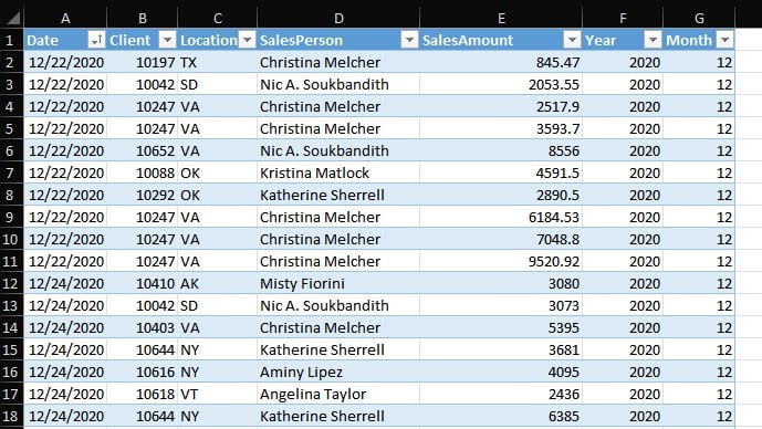
Consider an Excel file containing detailed sales data for a fictitious company. The dataset, organized in a Table named “Sales,” includes columns for Date, Client, Location, SalesPerson, and Sales Amount, along with calculated columns for Year and Month based on the Date field.
To calculate annualized total sales, you might traditionally use a PivotTable with the Year field in the Columns section and Sales Amount in the Data section to sum the values. With GROUPBY, you can achieve the same result dynamically using the following formula:
=GROUPBY(Sales[Year],Sales[SalesAmount],SUM)

This eliminates the need for manual PivotTable setup and provides a dynamic summary that updates instantly with changes to the dataset.
Dynamic Filtering with GROUPBY
GROUPBY also supports dynamic filtering, similar to PivotTables but with greater flexibility. For example, to view total sales by month, you can use this formula:
= GROUPBY(Sales[Month],Sales[SalesAmount],SUM)
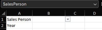
To introduce filtering capabilities, let’s assume you want to filter the data by Year and SalesPerson. First, add two dropdown cells to specify the desired filters, populated with unique values from the data using Excel’s Data Validation feature. Name these cells Year and SalesPerson for simplicity.
Next, incorporate these filters into the GROUPBY formula as follows:
=GROUPBY(Sales[Month],Sales[SalesAmount],SUM,0,0,1,(Sales[Year]=B2)*(Sales[SalesPerson]=SalesPerson))
This formula dynamically filters the data and displays the aggregated sum of total sales by month, based on the selected Year and SalesPerson, just like a PivotTable with filters.

Building Dynamic Charts and Visualizations with GROUPBY
One of the most powerful use cases of the GROUPBY formula is building dynamic charts and reports. By combining GROUPBY with Excel’s charting tools, you can create interactive visualizations that adjust automatically based on changes to the dataset or filters.
For advanced reporting, you can use this Excel file to build an online report with dynamic filters using SpreadsheetWeb. By converting your workbook into a web application, SpreadsheetWeb allows users to interact with the data in a browser, enhancing accessibility and collaboration. SpreadsheetWeb takes the power of GROUPBY beyond Excel, enabling businesses to create scalable, dynamic reporting solutions tailored to their needs.

GROUPBY is a game-changer for Excel users, offering the ability to create dynamic, formula-driven analyses and visualizations without the limitations of traditional PivotTables. Whether you’re summarizing sales data, building interactive dashboards, or integrating reports into web applications, GROUPBY provides the flexibility and efficiency to handle it all.


