Were you just handed a massive spreadsheet and you have no idea how it’s structured, or what it does? Are you tired of following the root cause of errors in your formulas? If you answered yes to any of these questions, or simply would like to learn formula auditing in Excel, then this guide is for you.
Formula auditing in Excel lets you see the relationship between formulas and cells from different perspectives. This can be extremely useful when you’re working with big files, or complicated, nested formulas. We need to start with the Formulas ribbon on Excel’s top menu, which contains all sorts of help tools for formulas.

Under this menu you can find a variety of tools that can help building and troubleshooting formulas in your workbook. We’re going to be focusing on the Formula Auditing features to the right of this menu.

To trace the roots of a formula, you can click on each cell and try following the formulas. However, this can be extremely time consuming, and especially hard if you’re not too familiar with the syntax structure of all formulas used.
Trace Precedents
The first feature in formula auditing menu, Trace Precedents, is designed to show all cells used in calculating the cell of your choice. When active, it will display the direction of cell references leading to that cell with arrows. Referenced cells and ranges will be marked with dots and boxes, respectively. A sheet icon means references from another sheet. You can download the example spreadsheet from here: Time Card - Formula Auditing.

If there are no trace precedents to the cell you’ve selected, you will receive an error message.

This is an extremely useful feature for creating a quick overview of the entire workflow in a spreadsheet. By identifying precedent cells, you can easily determine the purpose of a field.
Let’s see how this works with an example. Here we have a time card tool which was sent to us by the HR and we have no idea how it works. If we wanted to learn more about how it calculates the Total Pay, we can select this field, and press Trace Precedents from the Formula ribbon.
We can see that the Total Pay is calculated from hours Total and Rate/Hr. That’s a good start! Although it’s reasonable to think that the Total is calculated by adding the rows above it, let’s click Trace Precedents again to make sure.
Clicking Trace Precedents twice will highlight the preceding cells from one step before. This shows that the Total is derived from the Regular column where hour totals are added. Also, note that the Rate/Hr data is actually coming from another sheet (shown with a table icon next to it). How about the total hours, where do they come from? Let’s press Trace Precedents again and see how far back we can trace this logic.

Remove Arrows
Evidently, the Regular column adds and subtracts the Time In/Outs and gives the total hours worked. Trace Precedents feature can be used to track formulas as far as they go. However, overdoing this can complicate things, as things will get hard to see with arrows pointing in all directions. It’s recommended to choose a path and stick to it. To remove all arrows, click Remove Arrows in the same menu.

In this menu, select from the three options to avoid a congested look.

If the cell takes preceding values from another worksheet, this will be shown with a table icon. Double clicking the icon pointed by dashed arrows will bring the Go To window and display cell and range references.

Selecting an item in list and clicking OK will direct you to that cell.
Trace Dependents
What if we wanted to start from the end? The tools for formula editing in Excel also allow for tracing where a cell is used. Knowing the source of your formulas can help avoid deleting important references and unwanted #REF errors. To do this, select a source cell and press Trace Dependents. The arrows will point outwards and highlight cells or ranges referencing the selected cell.

Show Formulas
When you enter a formula to a cell, Excel automatically runs the calculations and displays the results. Ultimately, all you see is numbers and labels in every worksheet. Another useful feature for formula auditing in Excel, Show Formulas, allows you to reveal all formulas in your workbook. This will change the display from results, to their content to increase readability of the logic. To return to the regular view, press Show Formulas again.

Error Checking in Formula Auditing
Debugging large spreadsheets with tons of formulas can be a daunting task, but thanks to the Error Checking feature, you can quickly see if all formulas go all the way through.

The first (default) option, Error Checking, shows error in the spreadsheet and offers ways to debug them.

Show Calculation Steps will open a formula evaluation window, where you can find detailed information about the specific error.

You can select Ignore Error, Edit in Formula Bar, or navigate through all errors in the spreadsheet using the other buttons.
The next error checking feature, Trace Errors, works very much like Trace Precedents, but instead indicates errors with red arrows. Red arrows will only appear if there are errors in the formula.

The third option under Error Checking is the Circular References indicator. This handy list will show all cells in a circular reference loop. Click the cell name to go to it.

Evaluate Formula
Did you just see an extremely long, intimidating formula with nested arguments? Then the Evaluate Formula feature is for you. This tool solves complex formulas step by step.

Clicking this button will open a new window where you can follow formula logic. Each time you click the Evaluate button, Excel will solve the next underlined part of the formula, and show you the result.
Here is a quick example. We first click on the cell with the formula (here, we chose L6). The first cell reference is underlined.

Pressing Evaluate, previously underlined E6 cell’s value is replaced with reference. Next cell reference, F6, is underlined.
One thing to note here is that the next item is selected based on a few things like,
- Left-to-right
- Inner-to-Outer order of parentheses
- Mathematical operations order
- Logical order
- Inner-to-Outer order for nested functions
Previously underlined cell, F6, is found to be “30”. At this point; 30/60 operation takes priority because division comes before addition.
Press Evaluate again to conclude the division operation. Next is the sum operator. This can go on until the entire formula is resolved.
If the underlined part of the formula is a reference to another formula, press Step In to display the other formula in the Evaluation box. Click Step Out to go back to the previous cell and formula.

For example, formula in L16 is “=L13*L15”
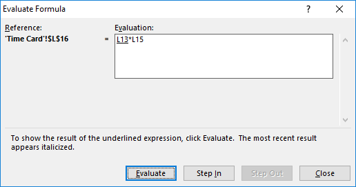
Clicking Evaluate returns value of “L13”. Using the Step In function, however, shows the formula syntax that returns the value of cell “L13” (The formula is “=SUM(L6:L12)”).

Please note that the Step In button will be disabled for a reference the second time it appears in the formula, or if the formula refers to a cell from a separate workbook.
Shortcuts for Formula Auditing in Excel
Here are some of the shortcuts to formula auditing features,
- Trace Precedents: Ctrl+[
- Trace Dependents: Ctrl+]
- Show Formulas: Ctrl + `
Thanks to tools for formula auditing in Excel, you don’t have to be intimidated by huge spreadsheets you come across! Be it for troubleshooting or analyzing a workbook, these tools can help identify key features and find errors in no time. Be sure to check our blog for more tutorials that can boost your Excel productivity!