Excel's Pivot Tables have revolutionized the way we handle and interpret data, facilitating easy management of vast amounts of information. Pivot Tables offer a streamlined and efficient approach to dissecting data, providing users with robust tools to summarize, explore, and present their datasets. However, like any tool, Pivot Tables have their limitations.
One of the primary limitations of Excel Pivot Tables is the handling of dynamic data. If the underlying data changes, Pivot Tables need to be manually refreshed to reflect these updates. This can be an inconvenience for datasets that change frequently. Although Pivot Tables offer a wide range of preset calculations, they may not accommodate complex or custom calculations as conveniently as Worksheet Formulas do. Pivot Tables have a predefined layout that may not always fit the specific presentation or reporting style users want. Although Excel provides some flexibility in design, Pivot Tables may not be the best choice for highly customized reports.
Microsoft Excel has been steadily improving its function library, introducing new dynamic array functions that can provide an alternative to traditional Pivot Tables. New functions such as SORT, FILTER, UNIQUE, SEQUENCE, XLOOKUP, LET, along with other Dynamic Array functions, enable Excel users to create complex data transformations and analyses that were previously only possible with Pivot Tables. However, unlike Pivot Tables, these functions automatically update to reflect changes in the underlying data. This article delves into how these innovative functions are redefining data analysis, providing alternatives to traditional Pivot Tables.
Create a Excel Pivot Table using Sales Data
Creating a Pivot Table with a simple sales data set in Excel is a straightforward process. Data should be in columns with clear headers. For example, a simple sales data set might include columns for "Date", “Sales Person”, "Product", and "Sales Amount".

Note that the example is in a well-organized data table form which each column contains a different set of values. Each row should represent a unique sales transaction. If your data set has multiple columns for same kind of data for example, different columns for product types, you should unpivoting your data first: How to Unpivot Data with New Excel Functions.
Creating a Excel Pivot Table from this data is as simple as selecting row and column fields in the "Create PivotTable" dialog box. ()
Pivoting Data with Excel Functions
Let’s go over how we can create the same pivot table using worksheet formulas. An Excel pivot table usually consists of 4 parts:
- Rows: Unique list of categories you need them as row headers.
- Columns: Unique list of categories you need them as column headers.
- Values: Aggregated values based on crossed row and column.
- Totals: Totals of values for each row and column including a grand total.
Let’s generate each part with individual formulas in Excel pivot table.
| Rows | =SORT( UNIQUE($J$7:$J$46)) |
Sorted list of Sales Person |
| Columns | =TRANSPOSE( SORT( UNIQUE($K$7:$K$46))) |
Sorted list of Products in horizontal form |
| Values | =SUMIFS( $L$7:$L$46, $J$7:$J$46,$P$7#, $K$7:$K$46,$Q$6#) |
Sum of values by relevant row and column label |
| Row Totals | =SUMIFS( $L$7:$L$46, $J$7:$J$46,$P$7#) |
Sum of values by rows |
| Column Totals | =SUMIFS( $L$7:$L$46, $K$7:$K$46,$Q$6#) |
Sum of values by columns |

Thanks to Excel’s array combining functions such as VSTACK and HSTACK, we can merge all these formulas into a single formula in Excel pivot table.
=VSTACK(array1,[array2],...)
=HSTACK(array1,[array2],...)
The VSTACK and HSTACK functions allow you to merge multiple arrays vertically and horizontally. However, we cannot simply combine arrays which are getting references from each other, such as values need row and column labels for filtering out.
However, this can be handled by using LET function and its formula-scoped named ranges. The LET function lets you define names within the scope of a formula. So, you can use names instead of references, preventing the need for repeated range selection. It makes formula writing and editing easier as well.
LET(name1, name_value1, calculation_or_name2, [name_value2, calculation_or_name3...])
In our example, references from the dataset are defined first.
  values,$L$7:$L$46,
  row_labels,$J$7:$J$46,
  col_labels,$K$7:$K$46,
Row and column labels follow them. Note that each formula uses the in-formula names instead of cell references: row_labels, col_labels.
  unique_row_labels,SORT(UNIQUE(row_labels)),
  unique_col_labels,TRANSPOSE(SORT(UNIQUE(col_labels))),
Next three definitions are for headers (column labels), calculations and totals. Each segment uses HSTACK function to combine columns. To provide empty columns, there are empty strings (“”) like in the header part.
  headers,HSTACK("",unique_col_labels,""),
  calculations,
  HSTACK(
    unique_row_labels,
    SUMIFS(values,row_labels,unique_row_labels,col_labels,unique_col_labels),
    SUMIFS(values,row_labels,unique_row_labels)),
  totals,HSTACK("",SUMIFS(values,col_labels,unique_col_labels),""),
Finally, the VSTACK function merges each segment vertically.
VSTACK(headers,calculations,totals)

=LET(
  values,$L$7:$L$46,
  row_labels,$J$7:$J$46,
  col_labels,$K$7:$K$46,
  unique_row_labels,SORT(UNIQUE(row_labels)),
  unique_col_labels,TRANSPOSE(SORT(UNIQUE(col_labels))),
  headers,HSTACK("",unique_col_labels,""),
  calculations,
  HSTACK(
    unique_row_labels,
    SUMIFS(values,row_labels,unique_row_labels,col_labels,unique_col_labels),
    SUMIFS(values,row_labels,unique_row_labels)),
  totals,HSTACK("",SUMIFS(values,col_labels,unique_col_labels),""),
  VSTACK(headers,calculations,totals))
What if the source dataset has empty rows? Then you will see 0 values for row and column labels, because Excel’s UNIQUE function evaluates those rows as well.

To eliminate these “empty rows” you can add a helper column to your dataset to determine which rows should be visible.
Our helper column formula checks the length of the string when columns are combined. If there is a character or more, the formula returns TRUE, otherwise FALSE.
=LEN(CONCAT(I7:L7))>0
Once the column is ready, the FILTER function in row and column labels definition can eliminate the empty rows.
=LET(
  values,$L$7:$L$106,
  row_labels,$J$7:$J$106,
  col_labels,$K$7:$K$106,
  unique_row_labels,SORT(UNIQUE(FILTER(row_labels,M7:M106))),
  unique_col_labels,TRANSPOSE(SORT(UNIQUE(FILTER(col_labels,M7:M106)))),
  headers,HSTACK("",unique_col_labels,""),
  calculations,
  HSTACK(
    unique_row_labels,
    SUMIFS(values,row_labels,unique_row_labels,col_labels,unique_col_labels),
    SUMIFS(values,row_labels,unique_row_labels)),
  totals,HSTACK("",SUMIFS(values,col_labels,unique_col_labels),""),
  VSTACK(headers,calculations,totals))

You can download the final Excel file from this link:
Turn Reporting Spreadsheets into Web Applications with SpreadsheetWeb.
Dynamic array formulas are integral to creating powerful reporting spreadsheets in Excel, enabling efficient dataset analysis and the extraction of valuable insights. Their potential is further enhanced when integrated into web-based applications, a task ideally suited for SpreadsheetWeb.
In this context, let's explore how an Excel file with pivot tables functions as a web application. While we won't cover the transformation process here, our website offers comprehensive resources on this topic. For detailed guidance on leveraging Excel pivot tablesl for web-based reporting applications, including transforming Excel files into web apps, we provide a wealth of articles and tutorials. The screenshot below illustrates the web application derived from the Excel file, showcasing its Excel pivot table functionality. Explore our site to learn more about utilizing Excel pivot tables effectively in Excel for web-based reporting and analysis.

As demonstrated in the video below, all calculations are instantly updated upon data entry, highlighting the benefits of employing worksheet formulas as opposed to Excel Pivot Tables.

Access Sales Sheet Application
In conclusion, the choice between using worksheet formulas and Excel Pivot Tables often hinges on the specific requirements of your data analysis task. While Excel Pivot Tables have traditionally been a powerful tool for summarizing and manipulating large data sets, the dynamic nature and flexibility of worksheet formulas, particularly with the advent of dynamic array functions, present a compelling alternative. These formulas enable real-time calculations, provide more customizability, and offer a degree of dynamism that static Excel Pivot Tables might not be able to match. That being said, Excel Pivot Tables still hold their own, especially when it comes to speed and ease of use for quick data exploration and analysis. Ultimately, as Excel continues to evolve and incorporate more advanced features, the ability to leverage both worksheet formulas and Excel Pivot Tables in harmony will likely be the key to efficient and effective data management and analysis.