If you don't want your users to see or be able to edit your formulas, you can lock, or hide them easily using Excel's Protect Sheet feature. This allows you to prevent any edits to formulas, or hide them altogether behind an optional password protection. Let us show you how to hide formulas in Excel using the Protect Sheet feature.

How to hide formulas in Excel

Protect Sheet feature can also be used to lock worksheets, but it doesn't hide the formulas by default. You need to select which cells are to be hidden before protecting your sheet. Here are the steps:

1. Select the cells containing formulas to be hidden.
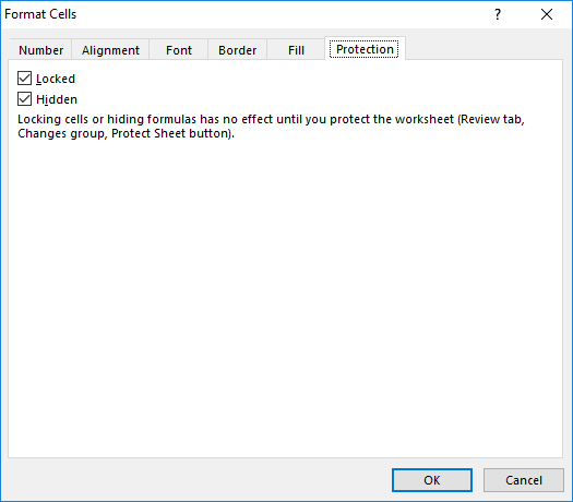
2. Press Ctrl+1 or right click and choose Format Cells… option to open the Format Cells dialog.
3. Go to the Protection tab.
4. Enable the Hidden checkbox.
5. Click OK to save your settings.
6. Protect your sheet from REVIEW > Changes > Protect Sheet button.
7. Enter a password. If you don't do this, users can simply click the Unprotect Sheet button to unlock the sheet.
8. Click OK to apply protection and hide your formulas.

The formula result will remain, but users won't be able to see the protected formulas.

You can also do this using number formatting!