Although the COUNTIF and COUNTIFS functions can count values by a given condition, they won't work if you want to use the output in other functions. In this article, we're going to show you how to count cells in Excel by year.
Syntax
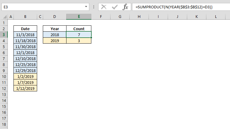
=SUMPRODUCT( N( YEAR( date values ) = year value ) )
Steps
- Start with the =SUMPRODUCT( function
- Use the N function, or double minus (--) signs to convert Boolean values into ones and zeroes N(
- Enter the criteria range – criteria condition by date and year numbers YEAR($B$3:$B$12)=D3
- Type in )) to close the N and the SUMPRODUCT functions, and finish the formula
How
The SUMPRODUCT function’s ability to handle arrays without array formulas provides an advantage over the limitations of COUNTIF and COUNTIFS functions. The SUMPRODUCT can evaluate and return arrays from range – value conditions. We use this functionality to run the YEAR function with array of date values and to resolve criteria range – criteria pairs.
YEAR($B$3:$B$12)=D3 returns {TRUE;TRUE;TRUE;TRUE;TRUE;TRUE;TRUE;FALSE;FALSE;FALSE}
The SUMPRODUCT function can sum the values in its argument array if there is only one argument. However, conditional equations return Boolean values, and therefore need to be converted into numbers which are meaningful for the SUMPRODUCT function. We can do this in two ways:
- The N function
- Double minus (--)
The N function converts a value to a number. In this case, TRUE and FALSE results will become 1 and 0. On the other hand, double minus operator will only work for this purpose, to return numbers from Boolean values. Either will work for this example.
N(YEAR($B$3:$B$12)=D3) returns {1;1;1;1;1;1;1;0;0;0}
As a result both, formulas below return the same values.
=SUMPRODUCT(N(YEAR($B$3:$B$12)=D3))
=SUMPRODUCT(--(YEAR($B$3:$B$12)=D3))