Identifying top values in a dataset can be efficiently accomplished using dynamic formulas. This guide will focus on how to use the LARGE function in Excel to highlight these significant values. We'll explore methods, including how to find the highest number in Excel, use Excel's LARGE function, and apply formulas to pinpoint and visually distinguish the largest values in a range.
Syntax of the LARGE Function
When using the LARGE function in Excel to highlight top values in a dataset, the formula you'll typically use is:
In this formula:
- Relative Cell Reference: This refers to the specific cell you're comparing against the top values in the dataset.
- LARGE Function: This key part of the formula is what makes the large function in Excel so useful. It finds the largest numbers in a specified range.
- Absolute Data Range Reference: This is the complete range of data where Excel is searching for the top values. It’s set as an absolute reference to remain constant even if the formula is copied to other cells.
- Top Value Count: Here, you specify the 'N' in 'top N' values you want to highlight. For instance, if you want the top 3 values, this parameter would be 3.
Steps to Highlight the Top Values in Your Dataset
- Select Your Data Range: Start by selecting the range of data in your table where you want to apply the highlighting.
- Access Conditional Formatting: Navigate to the 'HOME' tab on the Excel ribbon. Click on 'Conditional Formatting', then select 'New Rule' to open the conditional formatting options.
- Choose a Formula-Based Rule: In the 'New Formatting Rule' dialog box, select the option 'Use a formula to determine which cells to format'.
- Enter the LARGE Function Formula: In the provided space, enter the formula that includes the LARGE function. For example, =B2>=LARGE($B$2:$G$7,3). This formula compares each cell in your selected range to the third-largest value in the range from B2 to G7.
- Set Your Formatting Preferences: Click on the 'Format' button to open the 'Format Cells' dialog box. Here, you can choose how you want the top values to be highlighted — such as with a specific fill color, font color, or cell border.
- Apply and Confirm Your Settings: After setting your desired formatting, click 'OK' to close the 'Format Cells' dialog box, then click 'OK' again in the 'New Formatting Rule' dialog box to apply your conditional formatting.
By following these steps, you can dynamically highlight the top values in your dataset, making it easier to identify the highest numbers, like the Excel highest value in range" or find max value in excel, enhancing your data's visibility and interpretability.
How to Highlight the Top Values in a Data Set
Conditional formatting in Excel allows for automatic cell formatting based on specific criteria. Using the LARGE function in Excel, you can highlight cells within the top N values of a range. For example, the formula =B2>=LARGE($B$2:$G$7,3) will highlight the cell B2 if it's among the top 3 values in the range $B$2:$G$7.
This method relies on absolute references for the range (e.g., $B$2:$G$7) to remain constant and relative references for individual cells (e.g., B2) to adapt as the formula is applied across the range. This efficient approach automatically updates formatting without the need to adjust each cell manually.
For further insights, like ranking values, explore the RANK functions as detailed in our article on How to Rank Scores.