In Microsoft Excel, the Quick Access Toolbar (QAT) stands as a pivotal element, enhancing efficiency and ease of use. However, many users remain unaware of its full potential, primarily because certain indispensable features are not activated by default. This article will guide you on Excel's hidden commands, shedding light on how to customize the Quick Access Toolbar to suit your specific needs. From the basics of where to find the Quick Access Toolbar in Excel to advanced customization techniques, we aim to guide you through a journey of discovery and optimization. Whether you're looking to add the Find button, manage your Excel ribbon, or explore the depths of Excel's toolbar options, this guide is your quintessential resource for unlocking the true power of the Quick Access Toolbar in Excel.
What is Quick Access Toolbar (QAT)
Our exploration predominantly centers on the Quick Access Toolbar (QAT) in Excel, a remarkably versatile feature that offers a gateway to an array of hidden commands, not typically accessible on the Ribbon. This adaptability of the Quick Access Toolbar allows for the integration of nearly any command, providing a level of customization that truly enhances your Excel experience.
To unearth these hidden commands, one must navigate to the Excel Options. This can be accomplished through a simple pathway:
- Click on File, then Options, and finally, select Quick Access Toolbar.
Alternatively, for a more direct approach:
- You can right-click on any existing command on the QAT and choose to Customize Quick Access Toolbar.
This path not only reveals a treasure trove of hidden functionalities within Excel but also provides a straightforward method to tailor the Quick Access Toolbar to your specific workflow needs, whether it's adding the Copy button, adjusting the Excel menu, or personalizing the Ribbon.


How to Customize the Quick Access Toolbar (QAT)
Here's how you can customize this toolbar to better suit your needs in Excel step-by-step:
- Explore All Commands: Begin by selecting 'All Commands' from the dropdown menu. This action unveils an exhaustive list of available commands, far beyond the standard options seen in the Excel ribbon or toolbar.
- Personalize Your Selection: Browse through this comprehensive collection and pinpoint the commands that align with your workflow. Whether it's quick access to the 'Spell Check', 'Print Preview', or even specialized toolbars, you have the freedom to tailor your Quick Access Toolbar in Excel.
- Add Commands: After selecting your desired commands, use the 'Add' button to seamlessly transfer these features from the master list to your personal Toolbar. This step symbolizes the bridge between potential and practicality, enabling you to customize the toolbar to your liking.
- Finalize and Implement: With your chosen commands now listed on the right-hand side, representing your customized Toolbar, simply click 'OK' to save these changes. This action confirms your selections, integrating them into your Excel interface for quick and efficient access.

In addition to customizing the contents of the Access Toolbar in Excel, you have the flexibility to reposition it for optimal convenience and accessibility. If you prefer a more central location for the QAT, you can effortlessly relocate it below the Ribbon. This adjustment can be swiftly executed with a few simple clicks.
To do that, just right click anywhere within the Ribbon or the Toolbar itself. From the context menu that appears, select the option "Show Quick Access Toolbar Below the Ribbon". This action immediately shifts the Quick Access Toolbar from its default position above the Ribbon to a more prominent spot below it. This repositioning not only enhances the toolbar's visibility but also aligns it more intuitively with your workflow, making it easier to access and utilize the customized tools and commands you've added.

This layout can be especially useful for frequently-used features.
Double Underline, Strikethrough, Subscript and Superscript Features in QAT
In Excel, certain commands like Double Underline, Strikethrough, Subscript, and Superscript offer enhanced options for presenting data effectively. These features, while readily available, are often tucked away, not immediately visible in the standard Ribbon or Quick Access Toolbar.
To access these formatting tools, one can explore the Format Cells dialog.
Here's a brief guide to locating each of these commands:
Double Underline: A potent tool for emphasizing financial or important numerical data, the Double Underline command can be found within the Format Cells dialog. It adds an extra layer of underlining, offering a distinct way to highlight critical figures.
Strikethrough: Ideal for visibly marking items as completed or irrelevant without removing them, the Strikethrough command is also housed in the Format Cells dialog. This feature allows you to cross out text, maintaining a clear record while keeping the layout intact.
Subscript: For scientific data, chemical formulas, or mathematical expressions, the Subscript command plays a crucial role. Located in the same dialog, it enables you to format characters as smaller letters or numbers positioned below the regular text line.
Superscript: Similarly, the Superscript command is essential for mathematical equations, annotations, or referencing. Found alongside its counterpart, it allows for characters to be formatted as smaller text positioned above the normal line of type.

Document Location
A particularly handy yet often overlooked feature in Excel's Quick Access Toolbar (QAT) is the ability to quickly view or copy the file location of your current document. This functionality is immensely useful for efficiently managing and sharing file paths, especially in collaborative environments or complex directory structures.
Toto this, you need to integrate the 'Document Location' command into your Toolbar.
Access the Excel Options: Firstly, navigate to the Excel Options by following the path:
- File > Options > Quick Access Toolbar, or simply right-click on the QAT and choose 'Customize Quick Access Toolbar'.
Add the Document Location Command: Within the Excel Options, under the Quick Access Toolbar section, select 'All Commands' from the dropdown menu. Scroll through the list until you find the 'Document Location' command.
Customize Your QAT: Select the 'Document Location' command and click the 'Add' button to move it to your Quick Access Toolbar. This action places the command within easy reach, allowing you to instantly view or copy the file path of your Excel document.
Save and Apply: Click 'OK' to save your changes. Now, the Document Location command will appear on your Quick Access Toolbar, ready to be used whenever you need to quickly reference or share the location of your Excel file.

You can copy or enter a file's location and press Enter key to open that file.
Excel Options
Options under All commands gives you a shortcut to Excel Options.

You can also find commands for specific tabs under Options.

Calculation Options
Managing the way calculations are executed can significantly enhance efficiency, especially in large and complex files. The Quick Access Toolbar (QAT) offers an invaluable feature for this purpose: the integration of Calculation Options commands. By customizing the QAT to include these options, you gain control over when and how Excel performs calculations, a vital aspect for optimizing performance.
Consider adding specific commands for Calculation Options into your Toolbar. This customization enables you to switch between different calculation modes as per your requirements.
Here’s a detailed guide on how to do it:
Add Calculation Options to QAT: First, access the Excel Options by either following the path File > Options > Quick Access Toolbar or by right-clicking on the QAT and selecting 'Customize Quick Access Toolbar'. Here, you can choose to add the entire 'Calculation Options' command to the QAT. This command unfolds into a collapsible list, offering a compact yet comprehensive set of choices for calculation modes, including Automatic and Manual.
- Opt for Individual Commands: Alternatively, if you prefer more direct access, you can add individual calculation modes to the QAT. Specifically, you can place 'Automatic' and 'Manual' calculation options as separate commands on the toolbar. This approach provides immediate access to these frequently used settings, allowing you to swiftly toggle between automatic recalculations and manual control.
Customize for Efficiency: By incorporating these calculation options into your Quick Access Toolbar, you tailor Excel to your workflow's specific demands. In scenarios involving large datasets, opting for manual calculation prevents Excel from recalculating every time a change is made, thereby saving time and computational resources.
Save Your Customization: Once you've selected and added your preferred calculation options to the QAT, click 'OK' to save these changes. Your Quick Access Toolbar is now equipped with tools to manage Excel’s calculation modes effectively, ensuring a smoother and more controlled data processing experience.

Camera Tool Hidden Command
Excel's Quick Access Toolbar (QAT) can be transformed into a powerful tool for creating dynamic images of specific cell ranges or individual cells, enhancing navigation and efficiency when working with large sheets or data sets spread across multiple worksheets. This feature is particularly useful for swiftly moving between different parts of your workbook without the need to scroll or switch tabs repeatedly.
To utilize this innovative functionality, follow these steps to add and use the Camera command in your Quick Access Toolbar:
Integrate the Camera Command: Begin by customizing your Quick Access Toolbar to include the Camera command. Access the Excel Options by either navigating through File > Options > Quick Access Toolbar or by right-clicking on the QAT and selecting 'Customize Quick Access Toolbar'. From the list of available commands, choose 'Camera' and add it to your toolbar. This tool is a hidden gem for creating live images of your data.
Capture Your Data Range: Once the Camera command is part of your QAT, select the range or cell in your worksheet that you wish to mirror. This could be a set of cells, a chart, or any data segment you frequently refer to.
Activate the Camera Tool: Click on the Camera icon in your Toolbar. This action turns your cursor into a crosshair, ready to capture the selected range.
Create and Position the Dynamic Image: With the Camera tool activated, click and drag to create a rectangle where you wish the dynamic image to be placed. Once you release the mouse button, a live image of your selected range appears. This image is not just a static snapshot; it dynamically updates as the source data changes.

Email Attachment as a hidden command
Email command opens your default email client, create a new email with the latest version of your file is attached (with the file's active version saved).
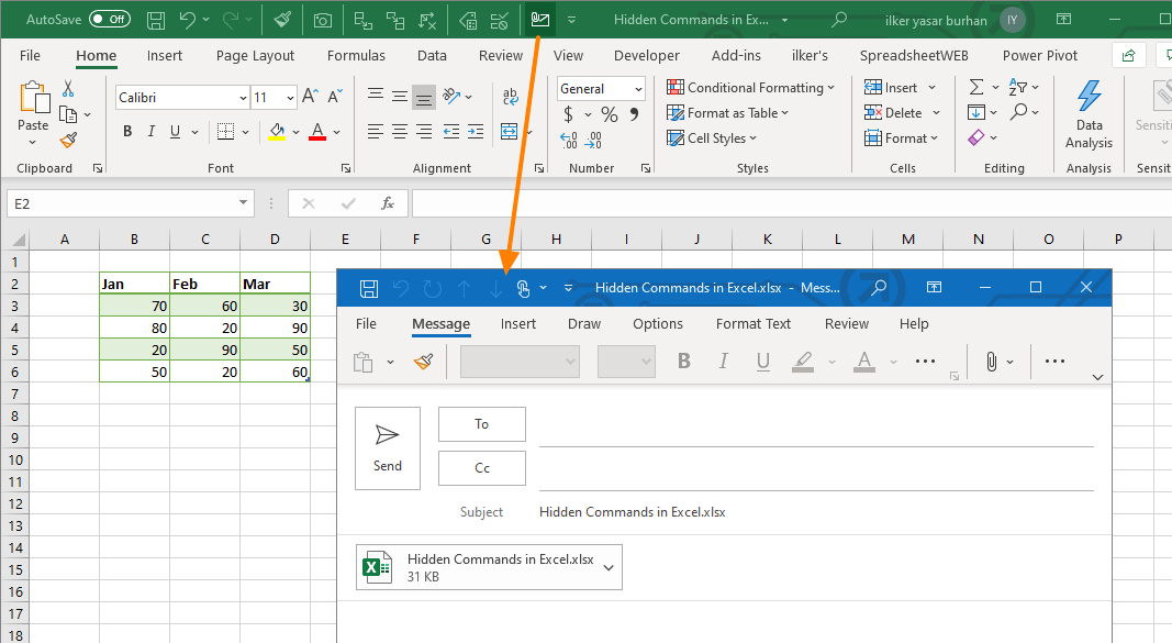
Commands are available for sending your file as a PDF or XPS.