Excel Just Changed Its Oldest Rule: One Cell Can Now Hold Many Values

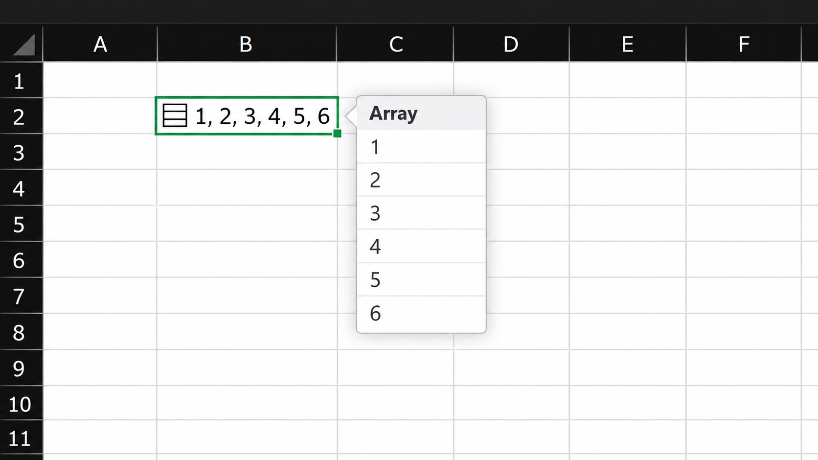
Since its introduction, Excel has held exactly one value in each cell. In a September 24, 2026 Microsoft 365 Insider announcement, Microsoft described a change to that model for Microsoft 365 Insiders on the Beta Channel for Windows and Mac. A cell can now contain a list, an array of any shape, or an array of arrays. The release includes four new functions, FLATTEN, HAS, HASANY and HASALL, and Microsoft advises against using the feature in production workbooks at this stage.

The stated purpose is to keep multiple related values, such as several owners of a project, in one cell while still allowing each value to be filtered and calculated on individually. The underlying change is broader than that. Arrays are now a value type that can be stored in a cell, referenced by formulas and returned as formula results, which has implications for the file format, calculation, compatibility with other versions of Excel, and workbook design.

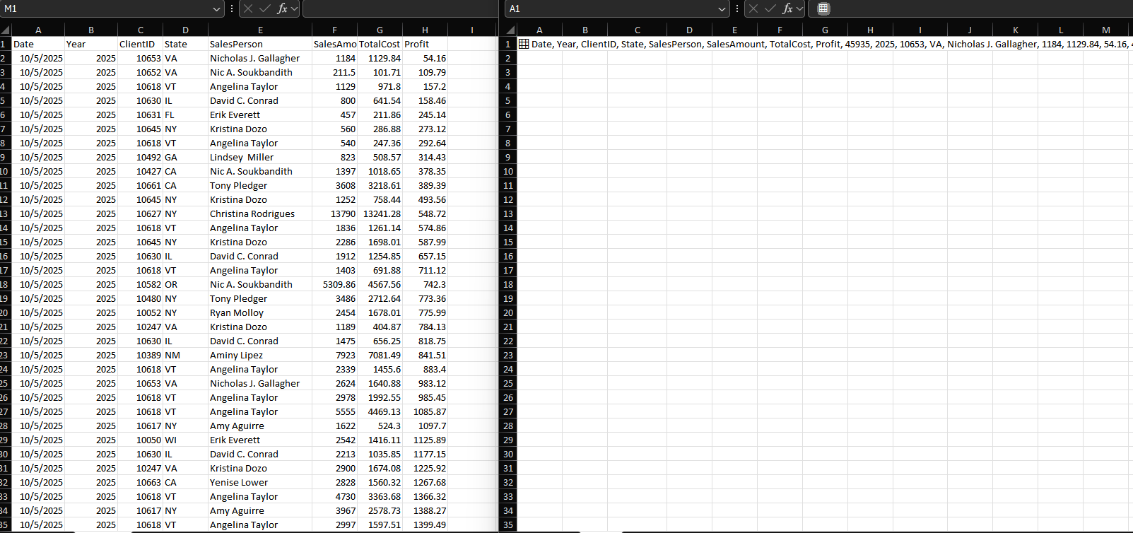
This article reports the results of testing the feature under realistic load rather than describing it from the announcement. We embedded a sales table of 12,785 rows and 8 columns (Date, Year, ClientID, State, SalesPerson, SalesAmount, TotalCost, Profit) in a single cell, did the same with a consumer complaints dataset of 322,301 rows and 14 columns, and derived a SalesPerson and States Operating table whose state lists each occupy one cell. We then examined the effect on the file, the behaviour in the current non-Beta build of Excel, the treatment by the formula engine, and the areas where the feature does not yet work. The tests were run in Excel Version 2610 (Build 20522.20000) on the Microsoft 365 Insider Beta Channel.

File size and storage

The first measurable effect concerns file size. When the 12,785-row sales table was moved from a conventional range into a single cell and the workbook saved, the file was approximately one third of its original size. The data and values were identical; only the storage location changed.

The cause is structural, and unzipping the workbooks makes it visible. In the range-based version of the sales table, xl/worksheets/sheet1.xml is 4,352 KB, because each value is written as a separate cell element carrying a reference, a type and a style, inside row elements. In the in-cell version, sheet1.xml is 2 KB and the data resides in a new part, xl/richData/rdarray.xml, at 1,519 KB. A single structured array replaces just over 100,000 tagged cell elements, at about 35 percent of the size. Repeating the comparison on the complaints dataset, 322,301 rows by 14 columns or about 4.5 million cells, gave a sheet1.xml of 156,172 KB against an rdarray.xml of 91,512 KB, a ratio of about 59 percent.

Dataset	Part	Flat range	In-cell array
Sales, 12,785 x 8	xl/worksheets/sheet1.xml	4,352 KB	2 KB
Sales, 12,785 x 8	xl/richData/rdarray.xml	not present	1,519 KB
Complaints, 322,301 x 14	xl/worksheets/sheet1.xml	156,172 KB	2 KB
Complaints, 322,301 x 14	xl/richData/rdarray.xml	not present	91,512 KB

The richData folder is where Excel already stores linked data types and images in cells, so the feature is built on the same rich-value infrastructure. Microsoft has not documented the format of rdarray.xml, but the file layout identifies the mechanism. A smaller file does not imply a smaller working set: Excel must still load the array into memory to calculate on it, and the on-disk size does not indicate how much memory that requires.

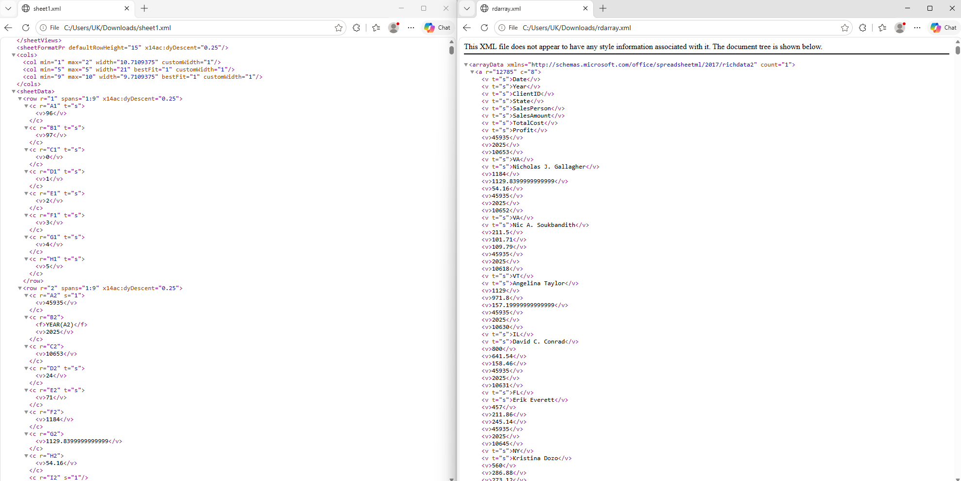
The two datasets indicate that the saving depends on the content. The sales table is predominantly numeric and reduced to about 35 percent of the original part size; the complaints table is predominantly text and reduced to about 59 percent. In a conventional sheet, repeated text is stored once in the shared string table and referenced by index from each cell, which keeps the per-cell cost of text low, and the array part does not appear to benefit from that indirection to the same degree. On the basis of these two measurements, an approximate expectation is a reduction to between one third and three fifths of the original size, with numeric data at the lower end of that range and text at the upper end.

Compatibility and interoperability

When the workbook is opened in the current, non-Beta build of Excel, the array cell displays #UNKNOWN!. This is the same error that linked data types produce in versions that predate them, and it indicates that the cell holds a value type the application does not recognise.

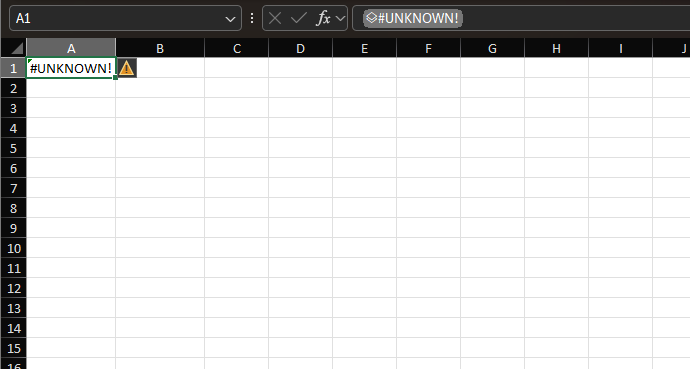
The round-trip behaviour is more favourable than the error suggests. After editing other cells in the older build, saving, and reopening the file in the Beta build, the array was intact. Copying the #UNKNOWN! cell and pasting it elsewhere in the older build, then saving and reopening, produced a copy that also contained the full array. The older build treats the cell as an opaque value that it can move and save without interpreting, and the rich-value parts survive the save. The data is not visible in that build, but it is preserved.

The array can be lost in one way. Pressing Delete on the #UNKNOWN! cell in the older build removes it, and it does not reappear when the file is reopened in the Beta build; no copy remains in the file. Because #UNKNOWN! resembles a broken formula, the principal risk when sharing such a workbook is accidental deletion by a user who does not recognise the value, rather than corruption.

Save As CSV writes only a small portion of the data, corresponding to the preview text displayed in the cell rather than the array behind it.

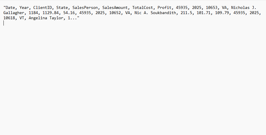
Within Excel, arrays move intact. Copying an array cell and using Paste Special > Values produces an array detached from its formula. This confirms that the array is a value rather than a display artefact, and it is the same property that allows the older build to carry it through a save.

Calculation performance and memory

The file size results show that the array is stored in a different structure from a worksheet range. Excel’s calculation engine was designed around ranges, so reading data from that structure may carry a cost that the on-disk figures do not reveal, both in recalculation time and in the memory required to hold the array once loaded. To test this, we used the 322,301-row consumer complaints dataset in two forms, as a conventional range and embedded in a single cell, and ran the same formulas against each.

Two formulas were tested against each layout. In the range workbook the data occupies A1:N322301 on a sheet named Consumer_Complaints; in the in-cell workbook the same data is stored as an array in Sheet1!A1. The in-cell versions use CHOOSECOLS on the array cell to obtain the columns the range versions reference directly: column 2 is Product, 6 is State, 8 is Submitted via and 13 is Timely response.

The first test used PIVOTBY with Product as rows, State as columns and a count of complaints, with headers, row and column totals, and rows sorted by total descending.

Range workbook:

=PIVOTBY(CHOOSECOLS(Consumer_Complaints!A1:N322301,2), CHOOSECOLS(Consumer_Complaints!A1:N322301,6), CHOOSECOLS(Consumer_Complaints!A1:N322301,1), COUNTA, 3, 1, -2, 1, 1)

In-cell workbook:

=PIVOTBY(CHOOSECOLS(Sheet1!A1,2), CHOOSECOLS(Sheet1!A1,6), CHOOSECOLS(Sheet1!A1,1), COUNTA, 3, 1, -2, 1, 1)

The second test used FILTER to return every row where State is CA, Submitted via is Web and Timely response is Yes.

Range workbook:

=FILTER(Consumer_Complaints!A1:N322301, (Consumer_Complaints!F1:F322301="CA")*(Consumer_Complaints!H1:H322301="Web")*(Consumer_Complaints!M1:M322301="Yes"))

In-cell workbook:

=FILTER(Sheet1!A1, (CHOOSECOLS(Sheet1!A1,6)="CA")*(CHOOSECOLS(Sheet1!A1,8)="Web")*(CHOOSECOLS(Sheet1!A1,13)="Yes"))

Each test was run in a fresh Excel session with no other Excel process running.

Each workbook was opened separately and timed with a VBA macro that performs five full recalculations with Application.CalculateFull and records each run. The timings therefore cover the whole workbook, which in each case contains only the data and the single test formula. The first run is reported separately and the remaining four are averaged. Memory was recorded as the Excel process’s Private Bytes after opening the workbook and after the fifth calculation.

The outputs were verified before timing. The FILTER result contained 27,874 rows and 14 columns in both layouts with the same first and last matching IDs, and the PIVOTBY grand total of 322,300 matched in both layouts.

Test	Layout	First run	Avg. runs 2 to 5	Private Bytes: open to final
PIVOTBY	Separate cells	1.633 s	1.599 s	197 to 763 MB
PIVOTBY	In-cell array	3.383 s	3.100 s	403 to 971 MB
FILTER	Separate cells	0.234 s	0.235 s	272 to 742 MB
FILTER	In-cell array	2.191 s	2.193 s	588 to 927 MB

The in-cell array was slower in every run. For PIVOTBY the average calculation time was 3.100 s against 1.599 s, a factor of 1.9. For FILTER it was 2.193 s against 0.235 s, a factor of 9.3. The FILTER test was repeated in two further sessions with results within 0.1 s of those shown.

The two ratios differ substantially, but the absolute differences do not. The in-cell PIVOTBY took about 1.5 s longer than its range equivalent, and the in-cell FILTER about 2.0 s longer. A fixed cost of that size added to a formula that takes 1.6 s on a range appears as a doubling; added to one that takes 0.2 s it appears as a tenfold increase. The measurements are therefore more consistent with a per-recalculation overhead of roughly 1.5 to 2 s associated with the 4.5-million-cell array than with the array path being uniformly slower per element. Because a full recalculation was used, part of that overhead may be the array cell itself being re-evaluated rather than the test formula reading from it; the present data cannot separate the two. The overhead may also scale with the number of references to the array cell, since the FILTER formula references it four times (once as the source and three times through CHOOSECOLS) and the PIVOTBY three times.

Memory shows a clearer difference. Immediately after opening, the in-cell workbook used 403 MB and 588 MB of Private Bytes in the two tests against 197 MB and 272 MB for the range workbook, suggesting that the array is loaded in full on open and held in a less compact form in memory than on disk. After five calculations the in-cell workbook remained higher in both tests, at 971 MB and 927 MB against 763 MB and 742 MB. Private Bytes measures the whole Excel process at the sampling points, not the array’s own allocation or the peak during calculation, so these are indicative of this setup rather than general figures. Taken together with the file size results, the picture is a format that is smaller on disk and larger in memory.

Independently of the timings, the tests confirmed that the array cell participates in Excel’s standard calculation chain. With manual calculation enabled, cells dependent on the array received the stale-value strikethrough that Excel applies to out-of-date results, in the same way as dependents of an ordinary range. The dependency engine treats the array cell as a normal precedent.

Functions and semantics

The formula engine is the most complete part of the feature. Every dynamic array function tested treated the in-cell table as an ordinary range.

CHOOSECOLS and DROP slice it. ROWS and COLUMNS return its dimensions. SORT, FILTER and UNIQUE operate on it directly. GROUPBY and PIVOTBY accept the cell as their source, with header detection and totals, so a summary of the 12,785-row table can be written in one line:

=GROUPBY(CHOOSECOLS(A1,4), CHOOSECOLS(A1,6,7,8), SUM, 3, 1)
=PIVOTBY(CHOOSECOLS(A1,5), CHOOSECOLS(A1,4), CHOOSECOLS(A1,6), SUM, 3, 1, 1, 1, 1)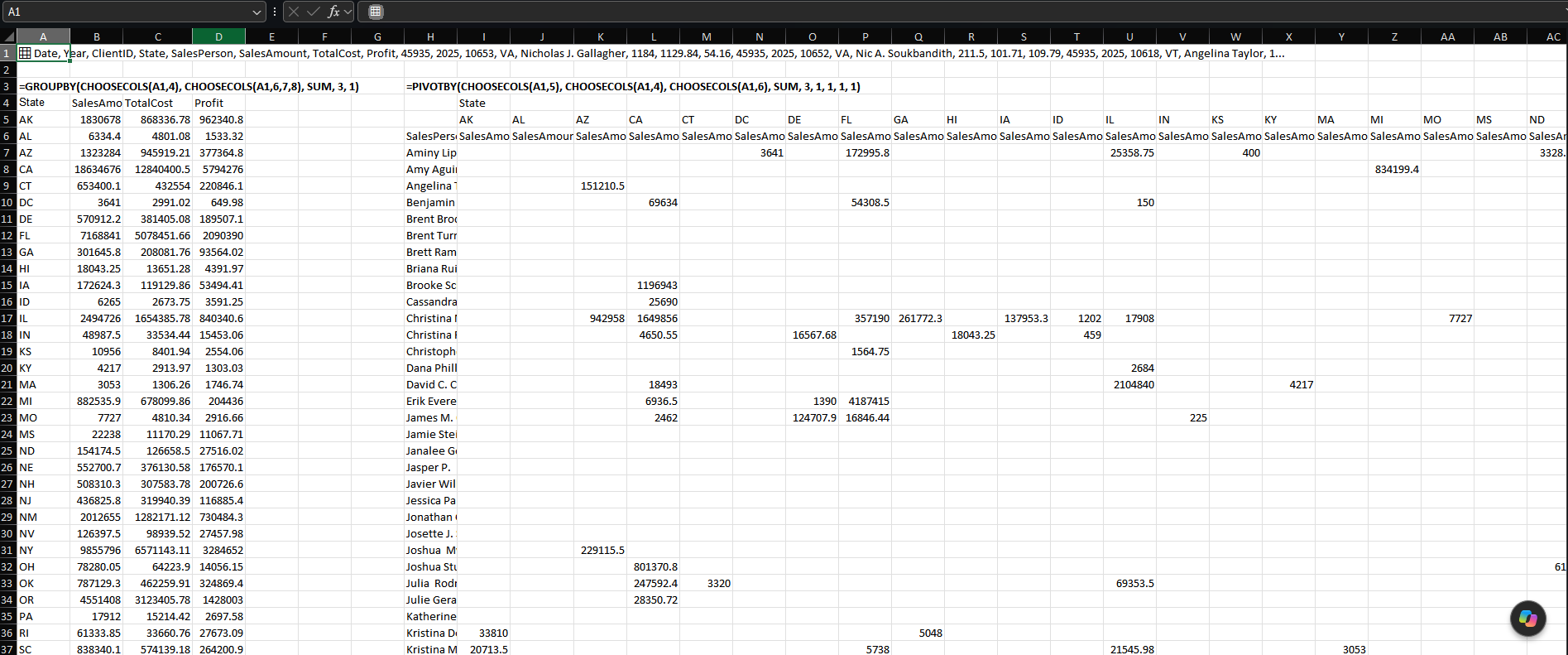

GROUPBY and PIVOTBY applied directly to the in-cell sales array.

The LAMBDA helper functions also worked with the in-cell sales array. BYROW calculated a profit margin for each data row, BYCOL produced column summaries, and SCAN calculated running sales totals. After excluding the header row, a BYCOL test identified the eight columns as number, number, number, text, text, number, number, number, matching the source data. This test checks the first data value in each column rather than every value. Dates retained their underlying numeric values, but the array cell did not carry over the original date formatting: a date could appear as its Excel serial number, such as 45935, until formatted as a date.

The column-profile formula was:

=BYCOL(DROP(A1,1),LAMBDA(c,IF(ISNUMBER(INDEX(c,1)),"number","text")))

BYCOL identifies the types of the first data row; the date appears as a serial number in the array preview.

Comparisons are elementwise, as with any array. In the sales-person table, =B4="NY" compares each state inside the list in B4 and returns a list of Boolean values rather than a single TRUE or FALSE. To test whether a salesperson operates in New York, =HAS(B4,"NY") reduces that comparison to one result. HASANY and HASALL similarly test for any or all values in a set. For example, the following formula returns the names of salespeople whose lists include NY:

=FILTER(A4:A36,MAP(B4:B36,LAMBDA(l,HAS(l,"NY"))))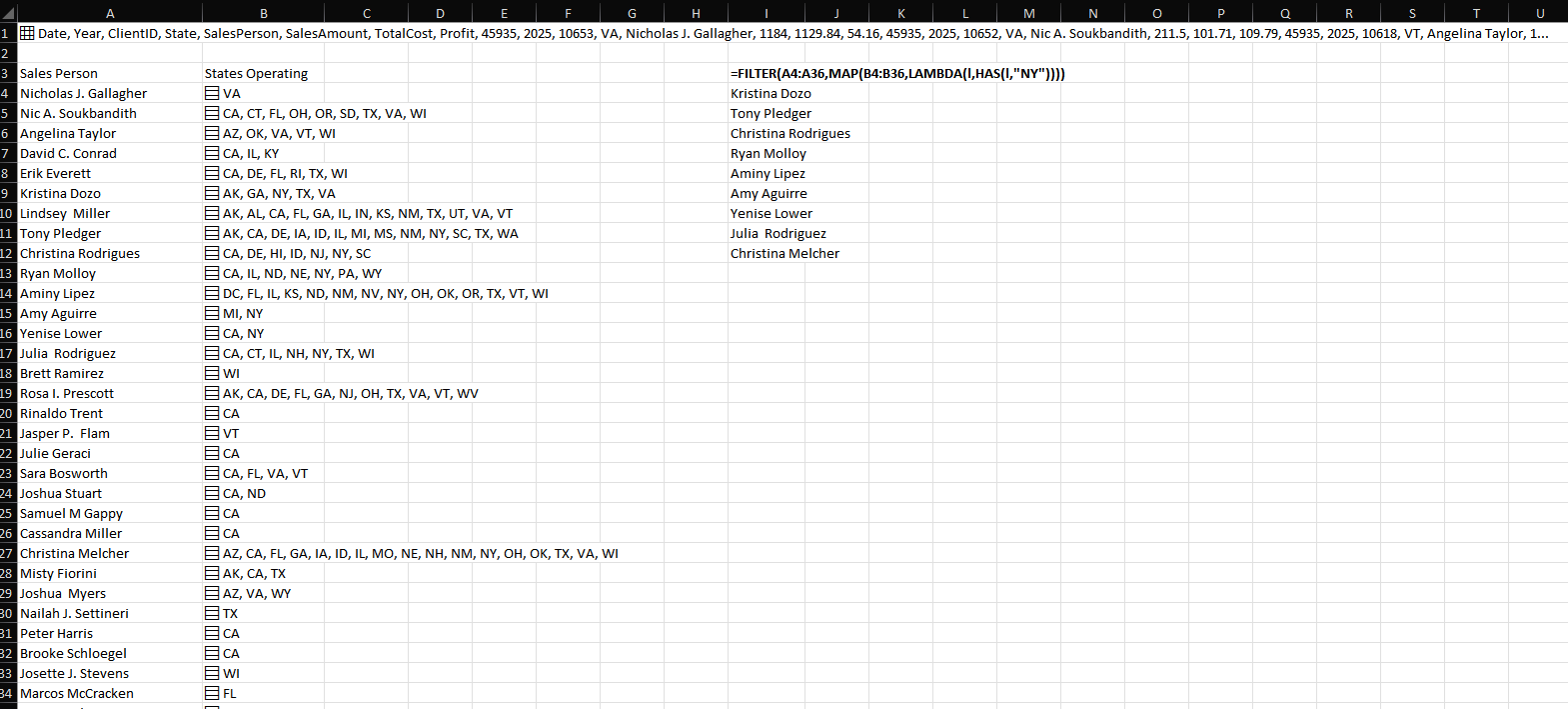

Salespeople whose state lists contain NY.

Updating data inside a cell

Loading data into a cell is straightforward, but changing individual items in an array cell is more limited. Microsoft lists Find & Replace’s inability to replace list or array items among the known limitations of this Beta release.

Formulas provide an alternative. To identify which salespeople operated in New York, using the state lists shown above:

=FILTER(A4:A36,MAP(B4:B36,LAMBDA(l,HAS(l,"NY"))))

To replace NY with New York in every list while keeping each result in its own cell:

=MAP(B4:B36,LAMBDA(l,{IF(l="NY","New York",l)}))

The exact-match IF is intentional. SUBSTITUTE matches substrings, so it could change a code embedded in a longer value. Comparing each list item with NY replaces only that code.

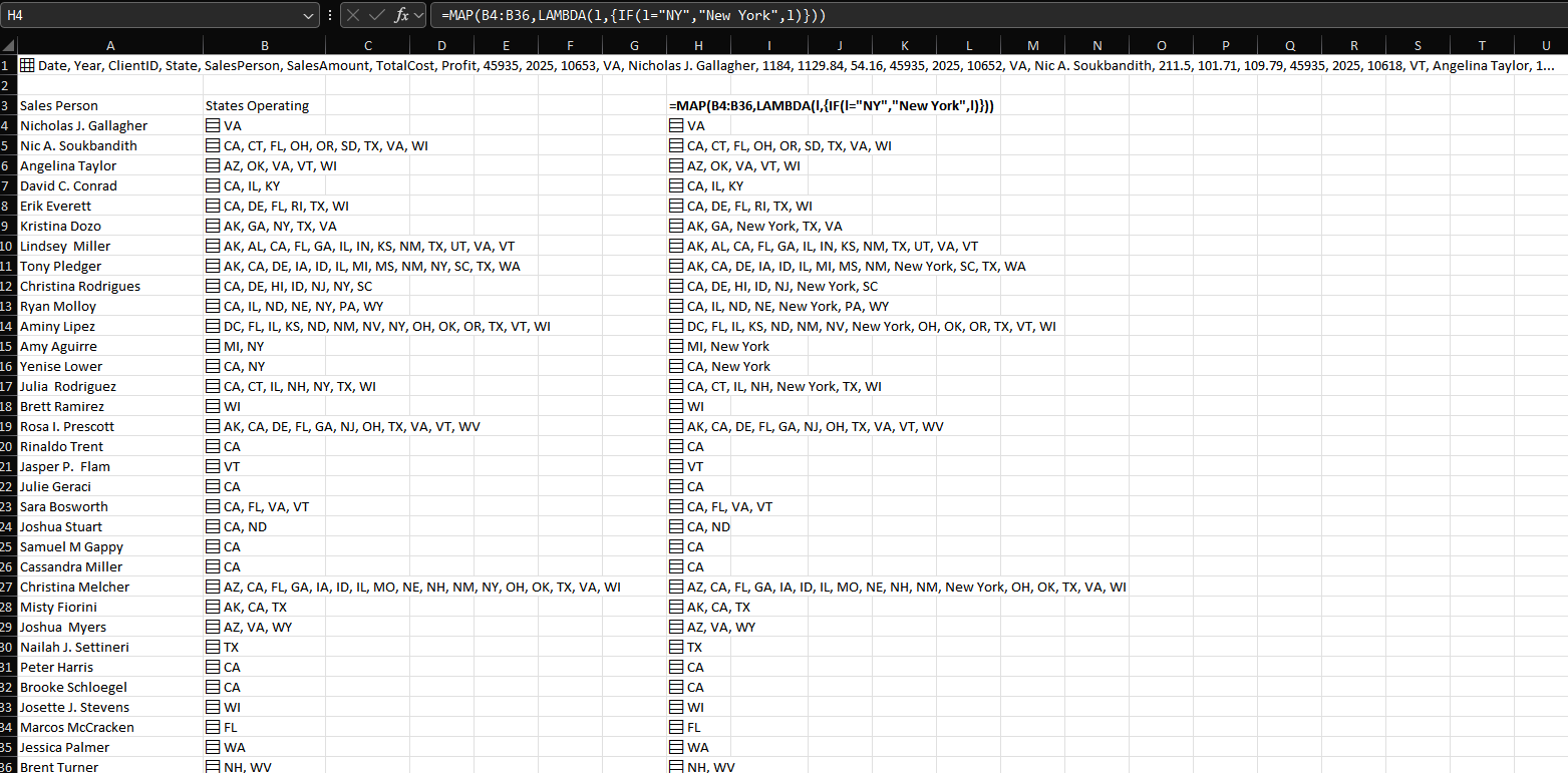
MAP returns a separate in-cell state list for each salesperson, replacing NY with New York.

The same approach applies to a complete table. Because the array is a value, an update is expressed as a new array derived from the existing one and kept in a cell with braces. Appending rows is a VSTACK:

={VSTACK(A1, NewRows!A2:H51)}

Modifying a single column requires rebuilding the table around it. The following formula increases SalesAmount by ten percent for Virginia while leaving the header row and the other columns unchanged:

={LET(t, DROP(A1,1), h, TAKE(A1,1),
  amt, CHOOSECOLS(t,6), st, CHOOSECOLS(t,4),
  VSTACK(h, HSTACK(CHOOSECOLS(t,1,2,3,4,5), IF(st="VA", amt*1.1, amt), CHOOSECOLS(t,7,8))))}

This approach is functional, but it is transformation rather than editing. There is no way to open the cell and change a single value in a specific row. Every change produces a new array, and the result is placed in a new cell unless it is pasted as values over the original.

Conclusion

In-cell arrays change what a cell can represent. In our tests, a single cell held a complete table that formulas could filter, group and transform, while list cells made multi-valued attributes usable without parsing text. The workbooks were smaller on disk, but the large in-cell array took longer to recalculate and used more process memory than the equivalent range. Editing, CSV export and use in older Excel builds remain practical limits for anyone considering this format for shared data.

These findings describe Excel Version 2610 (Build 20522.20000) on the Microsoft 365 Insider Beta Channel, using the workbooks and formulas described here. Beta behaviour, performance, file storage and compatibility can change before Microsoft releases the feature more broadly. The measurements and limitations in this article should therefore be treated as observations of this build, not predictions of the final release.