The FORECAST function is a Statistical function that predicts a future value by using existing values along with a linear trend (linear regression). You can use the forecasting function to predict future sales, inventory requirements, or consumer trends. In this guide, we’re going to show you how to use the FORECAST function and go over some tips and error handling methods.
Supported versions
The FORECAST function is supported across all versions of Excel.
FORECAST Function Syntax
x: This is the data point for which you want to predict a value. It represents the independent variable, and you are forecasting the y-value associated with this x-value.
known_y's: This is the set of known y-values or the dependent dataset. These are the data points that you have observed and are using to predict future values.
known_x's: This is the set of known x-values or the independent dataset. These values correspond to the known_y's and are used as the basis for the linear regression that predicts the future y-value for the given x.
FORECAST Function Examples
The FORECAST function predicts the value of data point x by given historical known_y's values and known_x's data points. It's important to ensure that the 'known_y's' and 'known_x's' ranges have the same number of data points; otherwise, the function will return an error. Additionally, the data should ideally have a linear relationship, as the FORECAST function is based on linear regression analysis.
The FORECAST function essentially fits a straight line through the known x- and y-values and then uses this line to predict the y-value corresponding to the new x-value you provide. This function is particularly useful in time series forecasting and trend analysis.
The equation for the FORECAST is![]()
where![]()
![]()
x = AVERAGE(known_x's)
y = AVERAGE(known_y's)
In this example, historical data is in the range B5:C19. To predict a value based on a new data point (B20), the FORECAST formula is applied as shown in the formula:

However, relying on a single forecasted value might not offer valuable insights. A more effective approach involves generating forecasts for multiple points and then visualizing these forecasts, usually through a line chart, to observe the trend. This process entails creating additional data points and replicating the formula while being mindful of absolute and relative references. This is crucial to maintain the integrity of the historical data ranges.

An interesting aspect to note is how the last historical data point is often mirrored in the forecast data (as seen in cell D19, for instance) to seamlessly connect the forecasted trend line with the historical data in the graph.
Error Handling in FORECAST Function
The FORECAST function can return errors under specific circumstances, and recognizing these can assist in troubleshooting. Here are some common errors and their causes:
#N/A Error: This is probably the most common error associated with the FORECAST function. It occurs if:
- The arrays known_y's and known_x's have different lengths.
- Either the known_y's or known_x's arrays are empty.
- The function is unable to find a match for the x value within the range of known_x's.
#VALUE! Error: This error appears if non-numeric values are included in the x, known_y's, or known_x's arguments. It also occurs if the x argument is not a number. It's essential to ensure that the x value is numeric since the FORECAST formula is designed to work with numerical data.
#DIV/0! Error: Although less common in the FORECAST function, this error might occur if the variance of your known_x's data is zero. In simpler terms, if all your known_x's values are the same, the function cannot perform a linear regression, leading to this error.
To mitigate these FORECAST formula errors, follow the best practices listed below:
- Data Validation: Make sure all data points in known_x's and known_y's are valid numeric values. Remove or correct any non-numeric values.
- Equal Array Sizes: The arrays for known_x's and known_y's must be of the same size. Always verify that they have an equal count of data points.
- Check for Empty Arrays: Ensure that neither known_y's nor known_x's is empty. A range with no data will immediately cause an error.
- Diverse Data Points: Avoid having all data points in known_x's being the same, as it impedes the linear regression calculation.
- Use of Appropriate Functions: For Excel 2016 and later versions, it’s recommended to use FORECAST.LINEAR instead of FORECAST. Though they are essentially the same, FORECAST.LINEAR formula is more current.
Other Excel Forecasting Functions
In Excel, apart from the basic FORECAST function, there are several other functions under the FORECAST family, particularly introduced in Excel 2016 and later versions. These functions are designed to handle different types of forecasting scenarios and data patterns.
FORECAST.LINEAR Function
FORECAST.LINEAR function is essentially the same as the classic FORECAST function. It predicts a future value using linear regression. The syntax is
=FORECAST.LINEAR(x, known_y's, known_x's)
It's recommended for use over the older FORECAST formula for linear forecasting in Excel 2016 and later versions. The introduction of FORECAST.LINEAR formula was part of an effort to streamline function names and make their purposes more intuitive. The ".LINEAR" suffix explicitly indicates that the function is performing a linear forecast.

FORECAST.ETS Function
FORECAST.ETS function stands for "Exponential Triple Smoothing." It's used for forecasting data with a seasonal pattern. The ETS algorithm can handle seasonal patterns and trends, making it suitable for more complex forecasting scenarios. The syntax is
=FORECAST.ETS(target_date, values, timeline, [seasonality], [data_completion], [aggregation])
One of the key strengths of the FORECAST.ETS function is its ability to automatically detect and adapt to the seasonality in the data, a feature not present in the simpler FORECAST.LINEAR formula. This makes it particularly useful in fields like retail sales forecasting, energy consumption analysis, and any other area where seasonal fluctuations are a defining characteristic of the data. The function applies a model that can account for trends (both increasing and decreasing), seasonal cycles, and the smoothing of irregularities in the data, providing a more nuanced and potentially accurate forecast than models that only consider linear trends.

FORECAST.ETS.SEASONALITY Function
FORECAST.ETS.SEASONALITY function returns the length of the seasonal pattern detected by Excel's FORECAST.ETS algorithm. It's useful for understanding the seasonal behavior of your data. The syntax is
=FORECAST.ETS.SEASONALITY(values, timeline, [data_completion], [aggregation]).
The main advantage of using the FORECAST.ETS.SEASONALITY formula lies in its ability to automate the detection of seasonality within a dataset, a task that can be both complex and nuanced when performed manually. This automatic detection is particularly useful in scenarios where the seasonality is not immediately apparent or when dealing with large datasets where manual analysis would be impractical. The function employs advanced algorithms to analyze the periodicity and intensity of seasonal patterns, making it a valuable tool in fields like retail (for predicting seasonal sales), meteorology (for weather patterns), and even in finance (for analyzing seasonal trends in markets).

FORECAST.ETS.CONFINT Function
FORECAST.ETS.CONFINT function provides a confidence interval for the forecast value at a specified target date. This is useful for understanding the range in which the actual value is likely to fall. The syntax is
=FORECAST.ETS.CONFINT(target_date, values, timeline, [confidence_level], [seasonality], [data_completion], [aggregation])
The main advantage of using the FORECAST.ETS.CONFINT formula is its ability to not only forecast future values but also to provide a range within which these values are likely to fall, with a specified level of confidence. This is particularly important in fields like financial planning, inventory management, and strategic planning, where understanding the uncertainty associated with forecasts can significantly impact decision-making. The function's output, a confidence interval, offers a quantified estimate of the potential accuracy of the forecast, allowing users to assess the risk and make more informed decisions.

FORECAST.ETS.STAT Function
FORECAST.ETS.STAT function returns a statistical value, such as the Alpha, Beta, Gamma, MASE, SMAPE, MAE, or RMSE, associated with the ETS algorithm used in FORECAST.ETS. It's helpful for analyzing the accuracy and parameters of the ETS model. The syntax is
=FORECAST.ETS.STAT(values, timeline, [statistic_type], [seasonality], [data_completion], [aggregation])
Using the FORECAST.ETS.STAT formula allows for a detailed analysis of the ETS forecasting model, providing insights into how the model is interpreting and weighing the historical data. By accessing key statistical measures, users can assess the model’s accuracy and sensitivity. For instance, parameters like Alpha, Beta, and Gamma represent the weights given to the level, trend, and seasonal components in the ETS model, respectively. Understanding these weights can help in fine-tuning the model for better accuracy. Meanwhile, error metrics like MASE (Mean Absolute Scaled Error), SMAPE (Symmetric Mean Absolute Percentage Error), MAE (Mean Absolute Error), and RMSE (Root Mean Squared Error) provide a quantitative measure of the model's prediction accuracy, helping analysts in validating the model’s effectiveness and comparing different models.