This article explains the process of to convert Excel columns to rows, commonly known as "unpivoting," using VLOOKUP formula. Unpivoting is the opposite of pivoting data (see Pivot Tables) by distributing values from a single column to multiple columns while keeping unique values in an anchor column. Understanding this transformation is important for efficiently organizing and analyzing data in Excel, offering insights into why such a conversion might be essential.
Transforming Excel columns into rows, or unpivoting, serves a critical role in data analysis and management. It allows for a more structured and comprehensible representation of information, making it easier to perform various analytical tasks. Unpivoting is particularly valuable when dealing with datasets where information is more naturally organized in a row-wise format rather than a column-wise arrangement. By adopting this approach, users gain enhanced flexibility in data manipulation and visualization.
Central to the unpivoting process is the VLOOKUP formula, a powerful tool in Excel. VLOOKUP, short for "vertical lookup," is employed to search for a specific value in a vertical column and retrieve corresponding data from another column. Its application in unpivoting involves referencing a unique identifier (anchor column) and extracting associated values, contributing significantly to the efficient transformation of data from columnar to row-based structures.
Syntax
Now, let's explore how to implement unpivoting using the VLOOKUP formula to convert excel columns to rows
Unique lookup value =lookup value & COUNTIF(expanding range of lookup values, lookup value again)
=VLOOKUP(Unique lookup value, table we look for, column number of where data is, 0 or FALSE for exact match)
Steps
- Add a new column at left of your table and select its first cell
- Type the formula that generates a unique value =E3&COUNTIF($E$3:E3,E3)
- Copy down the formula to the entire column
- Write numbers from 1 to maximum number for a unique value into rows as titles of a new table 1, 2, 3
- Write anchor values in the first column of the new table Panama City, Gainesville, Valdosta
- In VLOOKUP function, use combination of anchor values and order numbers to replicate the unique values in the main table =VLOOKUP($B16&C$15,$B$3:$D$10,2,0)
- Wrap the function with IFERROR to remove #N/A errors =IFERROR(VLOOKUP($B16&C$15,$B$3:$D$10,2,0),"")
How to Convert Excel Columns to Rows
In order to convert Excel columns to rows, the first step involves generating unique values for the VLOOKUP function. To ensure uniqueness, we use COUNTIF function. You can also use COUNTIFS because we only need single criteria and both work with the same logic. The trick is to use an expanding range ($D$3:D3). The expanding range uses mixed references (absolute and relative) to expand from an anchor cell when you copy it down.
By applying the COUNTIF function with an expanding range, running count values are produced with each additional row. The fusion of actual values (e.g., location names) with running count numbers results in unique values (e.g., Gainesville1, Valdosta1, Valdosta2, etc.), suitable for implementation with VLOOKUP.
=D3&COUNTIF($D$3:D3,D3)
Next step is to create titles for the new table. We mimic unique values by merging titles to use in VLOOKUP.

The final step is to use the VLOOKUP function to convert excel columns to rows, but with unique values this time. So, do not forget to merge the index number with actual lookup value before using VLOOKUP. The unique values are the combination of column values and row values. It is important to lock column reference for column titles while doing the same for rows.
=VLOOKUP($B16&C$15,$B$3:$D$10,2,0)
Additionally; we advise to wrap the formula with the IFERROR function to eliminate any #N/A! errors.
=IFERROR(VLOOKUP($B16&C$15,$B$3:$D$10,2,0),"")