Case sensitive count can not be handled easily using standard count formulas like COUNTIF or COUNTIFS. In this article, we'll shot you how you can count case sensitive data by using a combination of SUMPRODUCT and EXACT functions.
Syntax
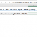
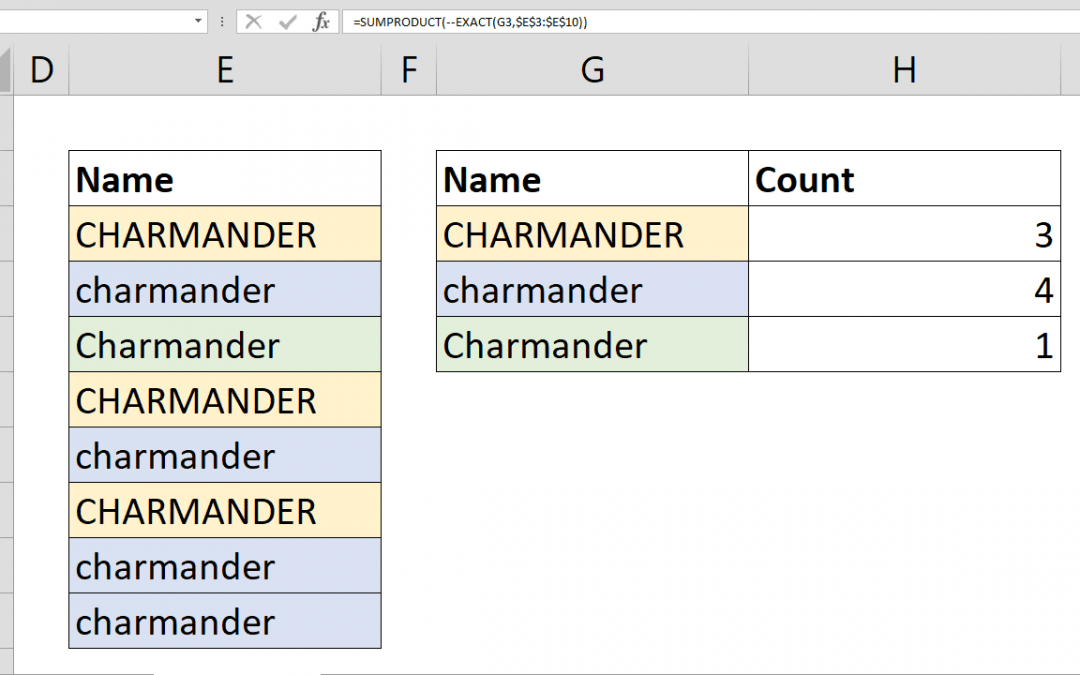
=SUMPRODUCT(--(EXACT(G3,$E$3:$E$10)))
Steps
- Start with =SUMPRODUCT(
- Type double minus characters to convert Boolean to numbers --
- Continue with EXACT(
- Select the reference that contains value to count G3,
- Select the reference that contains the range to be searched $E$3:$E$10
- Type )) and press Enter to close both functions and finish the formula
How
The regular COUNTIF or COUNTIFS functions don't support for case sensitivity as the other statistical functions in Excel. However, with SUMPRODUCT and EXACT functions, we can mimic case sensitive count. The EXACT function compares 2 strings and returns a Boolean value according to if they are "exactly" the same or not. In short, the EXACT function is case sensitive. There are 3 tricks we will use here:
- First, make the EXACT function return an array which is handled automatically when we defined our formula as an array formula.
- Second, convert TRUE/FALSE values into 1/0 by double minus characters.
- Finally, sum 1/0 values to count TRUE values in the array returned by the EXACT function. Note that 0 values are neutral in a sum operation.
Let's analyze the formula.
EXACT(G3,$E$3:$E$10) formula returns {TRUE;FALSE;FALSE;TRUE;FALSE;TRUE;FALSE;FALSE} array for "CHARMANDER" value. By wrapping the formula with the SUMPRODUCT function, we ensured the evaluation of EXACT function for each cell in $E$3:$E$10 range.
If the SUMRODUCT function has a single argument, it sums the values in the argument. Because of TRUE/FALSE values are not additive, we need to convert them to numbers. Double minus characters will do the trick. TRUE and FALSE values become 1 and 0 respectively if there are -- characters in front of the array.
Alternatively, the N function can do the same trick as well.
As a result; --EXACT(G3,$E$3:$E$10) returns {1;0;0;1;0;1;0;0} array.
Summing up 1 and 0 gives the count of the matched values because 0's are neutral.
=SUMPRODUCT(--EXACT(G3,$E$3:$E$10))
Also see related articles how to sum values with OR operator using SUMPRODUCT with multiple criteria, how to calculate weighted average with SUMPRODUCT.