FINANCIAL MODELING
Financial modeling is a fundamental process in finance involving the creation of abstract representations (or models) of a company's financial performance. These models are constructed based on a combination of a company's historical, current, and projected financial information. The essence of financial modeling lies in its ability to forecast future financial outcomes by creating a detailed spreadsheet that encompasses the company's revenue, expenses, and earnings. This approach is pivotal for various purposes, including valuation, budgeting, forecasting, capital allocation, business strategy planning, and risk management. Financial modeling is a critical tool for strategic decision-making, enabling businesses to project future earnings, assess financial risks, and plan accordingly.
The widespread use of Excel in financial modeling is attributed to several key factors. Firstly, Excel offers unmatched flexibility and customization, allowing users to tailor models to specific business needs and adjust them easily as assumptions or conditions change. Additionally, its widespread familiarity in the finance community makes it a go-to choice; many professionals already have a strong grasp of Excel, reducing the need for extensive training in specialized software.
Furthermore, Excel's robust functionality, featuring extensive financial functions such as NPV, IRR, and PMT, is crucial for constructing detailed and accurate financial models. Its powerful data analysis tools, including PivotTables, charts, and conditional formatting, aid significantly in parsing large datasets and presenting information in an accessible manner.
Integration with other business tools and the ability to import data from various sources further enhance Excel's suitability for financial modeling. This compatibility ensures comprehensive and cohesive models incorporating various data inputs. Cost-effectiveness also plays a role; compared to more specialized financial modeling software, Excel is more accessible while offering a broad spectrum of features.
The advent of cloud-based platforms like Office 365 has introduced new dimensions of functionality to Excel, including real-time updates and collaboration capabilities. This advancement has further solidified Excel's position as a central tool in financial modeling.
Financial modeling is an essential component of modern finance and business strategy, and Excel is the preferred instrument for this task. Its blend of flexibility, functionality, and familiarity, coupled with its integration and data analysis capabilities, makes it an indispensable resource for financial professionals worldwide.
FINANCIAL MODELING FUNCTIONS
XNPV Function
One of the most crucial concepts in finance and financial modeling is Net Present Value (NPV), a fundamental metric for assessing profitability. NPV is the calculation determining the difference between the present value of cash inflows and outflows over a specified period. This measure is pivotal in financial modeling as it helps analysts and investors evaluate the profitability and viability of investments or projects by considering the time value of money.
Excel, a powerful tool for financial modeling, offers functions to calculate NPV, facilitating detailed financial analysis and decision-making. While Excel has an NPV function specifically designed for calculating the net present value of a series of periodic cash flows, it often doesn't align perfectly with real-world scenarios where cash flows are not always periodic. This is where financial modeling in Excel becomes more nuanced.
To address this, Excel provides a more versatile function known as XNPV. The XNPV function is particularly useful in financial modeling because it includes specific dates for each cash flow, making it a more comprehensive tool for real-world financial analysis. The ability to incorporate actual dates of cash inflows and outflows leads to more accurate and realistic financial models.
Syntax
The syntax for the XNPV function in Excel is =XNPV(rate, values, dates), where 'rate' is the discount rate applied to the cash flows, 'values' represent the series of cash inflows and outflows, and 'dates' correspond to the specific dates of each cash flow. This function's ability to handle non-periodic cash flows makes it an invaluable component in the toolkit of financial modeling, providing a more precise evaluation of investment opportunities.
In summary, understanding and utilizing Excel's NPV and XNPV functions is essential in financial modeling, particularly when dealing with complex investment scenarios. These functions enable financial analysts to create more accurate models that reflect the real-world nuances of cash flow timing, ultimately leading to more informed investment decisions and financial strategies.
Example

FV Function
The FV, or Future Value function in Excel, is an indispensable tool in financial modeling, answering a fundamental question: What will be the worth of a certain amount of money at a future date? This function is critical in financial modeling for projecting the growth of investments or the future value of assets. It calculates the future value of a current asset, taking into account not just the initial amount but also the impact of regular payments and an assumed growth rate over a specified period.
In financial modeling, the FV function allows analysts to estimate the future value of investments under various scenarios. This can include savings accounts, retirement funds, or any financial asset with regular contributions or growth over time. The function considers the compound interest effect, making it a vital tool in financial planning and investment strategy arsenal.
Syntax
The syntax for the FV function is =FV(rate, nper, pmt, [pv], [type]), where:
- rate: represents the interest rate per period.
- nper: is the total number of payment periods in the investment.
- pmt: is the payment made each period; it remains constant throughout the investment's life.
- [pv]:, which stands for present value, is optional and represents the total amount that a series of future payments is worth.
- [type]:, also optional, denotes when payments are due - at the beginning (1) or end (0) of each period.
For financial modeling professionals, the FV function provides a way to model future financial scenarios accurately. It helps assess the potential outcomes of different investment strategies and plan long-term financial goals. Whether calculating the expected growth of a retirement fund over several decades or projecting the future value of recurring investments, the FV function is a key component in effective financial modeling. Its ability to incorporate various elements like periodic payments, interest rates, and the timing of payments makes it a comprehensive tool for predicting future financial scenarios.
Example

Note: Optional type argument is omitted in the example above. This variable defines whether payments are due at the beginning of the period or the end. If type is omitted, it is assumed that payments are due at the end of each period.
XIRR Function
In financial modeling, the Internal Rate of Return (IRR) stands out as a crucial metric for evaluating the potential profitability of investments. The key aspect of IRR is its 'internal' nature, implying that the calculation is based solely on the inherent cash flows of the investment and does not account for external factors such as inflation or cost of capital. This self-contained approach makes IRR a valuable tool in financial modeling, providing a clear, isolated view of an investment's potential returns.
Excel, a staple in financial modeling, offers the IRR function specifically designed to calculate the internal rate of return for investments involving periodic cash flows. This function is instrumental in financial modeling for assessing the viability and attractiveness of projects or investments based on their expected cash flows.
However, in the dynamic world of financial modeling, where cash flows often don't occur at regular intervals, Excel's XIRR function comes into play. The XIRR function is tailored for scenarios where cash flows occur at varying dates, offering a more flexible and realistic analysis of investments. This function is particularly useful in complex financial models where cash flows are not uniform or periodic, allowing financial analysts to derive a more accurate internal rate of return that reflects the real-world irregularities of cash flow timings.
In essence, both IRR and XIRR functions in Excel are integral to financial modeling, enabling professionals to make informed decisions by estimating the profitability of potential investments with precision, whether the cash flows are periodic or not. Using these functions in financial models significantly enhances the depth and reliability of financial analysis, particularly in investment appraisal and portfolio management.
Syntax
= XIRR(values, dates, [guess])
Example

Note: Optional type argument is omitted in the example above. This parameter defines a number you think is close to the result. If omitted, it is assumed to be 10%.
MIRR Function
Excel's MIRR, or Modified Internal Rate of Return, is a sophisticated variation of the traditional Internal Rate of Return (IRR) tailored for more nuanced financial modeling. As its name implies, MIRR is an advanced tool in capital budgeting specifically designed to evaluate and rank various investment opportunities of equivalent scale. Unlike the standard IRR, the Modified Internal Rate of Return considers both the costs associated with the initial investment and the potential returns from reinvesting the cash flows generated by the investment.
In professional financial modeling, MIRR is particularly valuable because it provides a more comprehensive perspective on the profitability of investments. By incorporating the reinvestment of cash flows, MIRR offers a more realistic assessment of an investment's potential yield, making it an indispensable tool in business decision-making. The function calculates the modified internal rate of return for a series of periodic cash flows, considering both the time value of money and the additional profits from reinvestment.
This dual consideration makes MIRR a preferred choice in sophisticated financial models, especially when comparing investment options with similar capital outlays but differing cash flow profiles. Its application is crucial in guiding strategic investment decisions, enabling financial analysts and business professionals to pinpoint the most financially viable opportunities. The MIRR function, therefore, is not just a computational tool but a strategic asset in capital budgeting and investment analysis.
Syntax
= MIRR(values, finance_rate, reinvest_rate)
Example

PMT Function
In financial modeling, the PMT (payment) is one of the most recognized and utilized tools. This function is specifically designed to calculate the value of payments for a loan characterized by constant payments and a steady interest rate. A critical aspect to note in financial modeling is that the payment value generated by the PMT function encompasses both the principal and interest components of the loan. This comprehensive approach makes the PMT function an essential component in the financial analyst's toolkit, providing a clear understanding of the periodic financial obligations associated with various loan structures.
Syntax
= PMT(rate, nper, pv, [fv], [type])
Example

Note: You may have noticed that the calculated payment amount is negative. This is because of the direction the money is going. Removing the dash (-) or multiplying the result with ‘-1’ returns the value as positive.
PPMT Function
In financial modeling, the PPMT function emerges as a specialized variation of the well-known PMT function. Designed to calculate the principal portion of a payment for a specific period, the PPMT function is vital in analyzing investments that involve periodic, constant payments and a steady interest rate. A key feature of this function is the inclusion of an additional parameter, known as 'per,' which specifies the exact period for which the principal payment is calculated. Within the context of the loan's term or investment period (nper), this 'per' parameter must be set to a value ranging from 1 to nper, enabling financial analysts to determine the principal repayment for any specified period. This precision makes the PPMT function an invaluable tool in detailed financial modeling, particularly when assessing the amortization of loans or the allocation of payments in investment planning.
Syntax
=PPMT(rate, per, nper, pv, [fv], [type])
Example
The example below shows the PPMT for the 10th month of the total 36 months payment period.

EFFECT Function
In financial modeling, the EFFECT function plays a pivotal role by providing an effective annual interest rate, which accounts for the impact of compounding within a specific period. This function is crucial for accurately determining financial products' real cost or yield in scenarios where compounding frequency differs from the standard annual rate.
Typically, interest rates in finance are quoted on an annual basis. However, when compounding occurs more frequently (e.g., monthly or quarterly), the effective annual interest rate is higher than the nominal or stated annual rate. This distinction is critical in financial modeling, affecting investment returns or loan cost assessment.
For instance, consider a loan with a nominal annual interest rate of 12.0%, compounded monthly. Although the rate is quoted annually, the monthly compounding elevates the effective annual interest rate to approximately 12.7%. This increase is due to the effect of 1.0% interest compounding each month, which, in aggregate, results in a higher overall annual rate.
Conversely, the NOMINAL function in Excel is a complementary tool in financial modeling. It calculates the nominal annual interest rate and the number of compounding periods from a given effective annual interest rate. Essentially, it reverses the process of the EFFECT function, providing insights into the stated annual rate when the effective rate and compounding frequency are known.
The EFFECT and NOMINAL functions are indispensable in financial modeling, especially for analyzing and comparing financial products or investments where the compounding frequency significantly alters the effective cost or yield beyond the nominal rate. These functions aid in presenting a more transparent and accurate financial analysis, essential for informed decision-making in finance.
Syntax
=EFFECT(nominal_rate, npery)
Example

RATE Function
In financial modeling, the RATE function in Excel is an essential tool for calculating the interest rate per period of an annuity. This function is adept at determining the specific interest rate necessary to amortize a loan over a designated time frame fully. Its application is particularly crucial in financial modeling scenarios involving structuring or analyzing loans and annuities, providing valuable insights into the interest obligations of various financial products.
Syntax
=RATE(nper, pmt, pv, [fv], [type], [guess])
Example

Note 1: The payment value is entered as a negative value because of the direction the money is going (i.e. out of pocket)
Note 2: The result represents the interest rate per period (i.e. month). Multiply the result by 12 to find the annual interest rate.
DB Function
DB stands for Declining Balance. This function calculates the depreciation expense of an asset for a specified period, using the ‘fixed-declining balance’ method.
Excel uses different calculations while calculating depreciation values at different periods. The rate is assumed to be 1 - ((salvage / cost) ^ (1 / life)) and is rounded to three decimal places.
- first period,
cost * rate * month / 12
- following periods,
(cost - total depreciation from prior periods) * rate
- last period,
((cost - total depreciation from prior periods) * rate * (12 - month)) / 12
Syntax
=DB(cost, salvage, life, period, [month])
Example

Note: The omitted Month argument is assumed to be 12.
SLN Function
The SLN (straight-line) function calculates an asset's ‘straight-line’ depreciation for one period. This method assumes that the cost of a fixed asset is reduced uniformly over the asset's useful lifespan.
The straight-line method is calculated like this:
(initial cost – salvage value) / lifetime
Syntax
=SLN(cost, salvage, life)
Example

We covered the 10 most common and useful formulas in financial modeling, but go ahead and experiment yourself! We hope this was a good place to start, or a refresher, to dive into doing finance with Excel!