Percentages are a fundamental concept in mathematics and everyday life, representing a number or ratio that signifies a fraction of 100. This representation is extensively utilized across various fields, from finance and economics, where it's employed to compute interest rates and assess risk, to a multitude of applications where emphasizing the contribution of a specific item to the whole is essential. In this article, we'll delve into the world of percentages, exploring what they mean and how to calculate them effectively in Excel. Additionally, we'll provide valuable tips and practical examples to help you grasp the concept and its practical application.
The concept of percentages revolves around the idea of expressing a part or portion of a whole in relation to 100. It allows us to compare and understand the relative size or significance of various elements within a dataset. For instance, in financial analysis, a percentage can represent the growth rate of an investment or the proportion of a budget allocated to specific expenses.

Standard Percentage Calculation
Percentages play a crucial role in expressing the relative size or significance of values in various contexts. The concept is rooted in our decimal (base 10) system, making it easy to calculate. To find the percentage representation of one value compared to another, all you need to do is multiply the ratio of the two numbers by 100. This formula can be represented as:
Percentage = (Numerator / Denominator) * 100
For instance, when you have 3 out of 4, you can express it as 75 out of 100, which simplifies to 75%. This straightforward calculation allows you to easily convey the proportion or contribution of a specific value within a larger context.
Excel simplifies the process of calculating percentages using basic arithmetic operations. Typically, you'll be determining the percentage that one value represents in relation to another. The formula for calculating a percentage in Excel is as follows:
Percentage = (Part / Whole) * 100
In this formula, 'Part' represents the specific value or portion you want to express as a percentage, and 'Whole' signifies the total or the context within which the part exists. By multiplying the result by 100, you obtain the percentage representation.
In the following sections, we'll provide practical examples and tips to help you master the art of calculating percentages in Excel for various scenarios.
How to Calculate Percentage in Excel
Calculating percentages in Excel can be made even simpler, eliminating the need to manually multiply the fraction by 100. Excel offers a convenient feature where you can directly apply a percentage number format to your cell containing the result, and Excel will automatically display it as a percentage value.
Here's the straightforward process:
- After entering your formula to calculate the percentage using the formula:
- select the cell where you want to display the result. Next, head over to the HOME tab and click on the '%' icon. Excel will then format the cell content as a percentage, instantly converting your fraction into a clear and easy-to-read percentage value.
- Alternatively, if you prefer more formatting options, you can access the 'Format Cells' dialog, where you can apply the percentage format just as you would with any other format type. This flexibility allows you to tailor the presentation of your percentage values according to your specific preferences and requirements.

Calculating Total Amount with a Given Percentage
Picture yourself shopping for a shirt that's priced at $15, with a tempting 25% discount. The question that arises is, "What was the initial price of the shirt?" To uncover the original price, you'll need to ascertain what figure represents 75% of the original cost, ultimately summing up to $15.
- Begin by selecting any vacant cell within your Excel spreadsheet.
- Input the formula `=15/0.75` and then press RETURN.
Result: The calculated value is 20, denoting the original price of the shirt.
- To format this result as currency, select the cell with '20' in it.
For recent Excel versions:
-
- Access the Home tab.
- Click on 'Number Format' and opt for 'Accounting' to display the result as '$20.00,' signifying the initial shirt price.
In Excel for Mac:
-
- Proceed to the Home tab.
- Under 'Number,' select 'Currency' to format the outcome as '$20.00.'
You retain the flexibility to adjust the number of decimal places in the result by clicking 'Increase Decimal' or 'Decrease Decimal' based on your preferences.
Raising a Number by a Percentage
Imagine your typical weekly food expenditure is $113, and you decide you want to boost your weekly food budget by 25%. In such a scenario, you need to calculate the new amount you can allocate for your weekly food expenses.
- Begin by selecting any vacant cell in your Excel spreadsheet.
- Input the formula `=113*(1+0.25)` and then hit RETURN.
Outcome: The calculated value shows as 141.25, indicating that you can now allocate $141.25 for your weekly food budget, reflecting a 25% increase.
- To format this result as currency, simply choose the cell containing '141.25.'
For recent Excel versions:
-
- Go to the Home tab.
- Click on 'Number Format' and opt for 'Accounting' to display the result as '$141.25.'
In Excel for Mac:
-
- On the Home tab, under 'Number,' select 'Currency' to format the outcome as '$141.25.'
You have the flexibility to adjust the number of decimal places in the result by clicking 'Increase Decimal' or 'Decrease Decimal' based on your preferences.
Reducing a Number by a Percentage
Now, envision a scenario where your weekly food allowance is $113, but you intend to decrease it by 25%. In this instance, you need to calculate your new weekly allowance.
- Begin by selecting any empty cell in your Excel sheet.
- Input the formula `=113*(1-0.25)` and then press RETURN.
Outcome: The calculated value reads as 84.75, signifying that your revised weekly food allowance is $84.75, reflecting a 25% reduction.
- To format this result as currency, select the cell containing '84.75.'
For recent Excel versions:
- Access the Home tab.
- Click on 'Number Format' and choose 'Accounting' to display the result as '$84.75.'
In Excel for Mac:
- Navigate to the Home tab, and under 'Number,' click 'Currency' to format the outcome as '$84.75.'
You have the flexibility to adjust the number of decimal places in the result by clicking 'Increase Decimal' or 'Decrease Decimal' according to your preferences.